Download
1 / 27
270 likes | 455 Vues
Optimal Rebalancing Strategy for Pension Plans A Presentation to State Street Associates 15.451 Financial Engineering Proseminar MIT Sloan School of Management November 18, 2004. Problem Summary. Managers create portfolios comprised of various assets

E N D
Optimal Rebalancing Strategy for Pension PlansA Presentation to State Street Associates15.451 Financial Engineering ProseminarMIT Sloan School of ManagementNovember 18, 2004
Problem Summary • Managers create portfolios comprised of various assets • The market fluctuates, asset proportions shift • Given that there are transaction costs, when should portfolio managers rebalance their portfolios? • Most managers currently re-adjust either on: • a calendar basis (once a week, month, year) • when one asset strays from optimal (+/- 5%) Both of these methods are arbitrary and suboptimal.
Why is this problem important? • An optimal rebalancing strategy would give a firm a measurable advantage in the marketplace • Providing rebalancing services could be a significant new revenue stream for State Street Getting this right would be worth lots (and we mean lots) of money
Presentation Outline • Simple Example • Our Solution • Methodology • Two Asset Model • Multi-Asset Model • Sensitivity Analysis • Conclusion • Future Research
A Simple Example • On Aug. 15 your portfolio was 50% invested in Nasdaq (QQQ) • You go on a three month, round-the-world trip • On Nov. 15 you waltz into the office, and realize your investment went up!!!
A Simple Example (cont.) • Sadly, the other 50% of your portfolio was invested in a long term bond fund (PFGAX) • Long term bonds have underperformed recently
A Simple Example (cont.) • Your portfolio is now unbalanced. • Should you rebalance now? • When should you have rebalanced? • What if the act of trading costs you 40 bps? • 60 bps? or a flat fee per trade? • Now imagine if you had many different assets, of all different types!!! • What about taxes? When and how to rebalance is complicated. Transaction costs make it much more difficult.
Our Solution • In theory when to rebalance is easy: Rebalance when the costs of being suboptimal exceed the transaction costs • In practice the transaction cost is known (assuming no price impact). • It is difficult to know the benefit of rebalancing.
When to rebalance depends on three costs: • Cost of trading • Cost of not being optimal this period • Expected future costs of our current actions The cost of not being optimal (now and in the future) depends on your utility function
Utility Functions • Quantify risk preference • Assume three possible utilities
Certainty Equivalents • Given a risky portfolio of assets, there exists a risk-free return rCE (certainty equivalent) that the investor will be indifferent to. • Example: 50% US Equity & 50% Fixed-Income ~ 5% risk-free annually • Quantifies sub-optimality in dollar amounts • Example: Given a $10 billion portfolio. • The optimal portfolio xopt is equivalent to 50 bps per month • A sub-optimal portfolio xsub is equivalent to 48 bps per month • On this portfolio, that difference amounts to $2 million per month
J2(r2) – expected benefit at time 2, given roll of r2 r3 • J2(r2) = max( r2, E(J3(r3)) ) = max( r2, 3.5 ) Roll r2 Roll • J1(r1) = max( r1, E(J2(r2)) ) r1 Accept if r2>3.5 Accept if r1>E(J2(r2)) Dynamic Programming - Example • Given up to three rolls of a fair six-sided die • Payout is $100 (result of your final roll) • Find optimal strategy to maximize expected payout Solution • Work backwards to determine optimal policy
Dynamic Programming • Examine costs rather than benefit • Jt(wt) is the “cost-to-go” at time t given portfolio wt Current period tracking error Cost of Trading Expected future costs • Trade to wt+1 (optimal policy) • When wt+1 = wt, no trading occurs
Assumed normal returns Data and Assumptions • Given monthly returns for 8 asset classes and table of expected returns • Used 5 asset model due to • computational complexity • lack of diversification in computed optimal portfolio
Optimal Portfolios • Calculated efficient frontier from means and covariances • Performed mean-variance optimization to find the optimal portfolio on efficient frontier for each utility
Two Asset Model • Demonstrate method first on simple two asset model • US Equity 7.06%, Private Equity 14.13% (2% risk-free bond) • 10 year (120 period) simulation
Multi-Asset Model • We construct the optimal portfolio from 5 of the 8 assets • Some assetswere highly correlated with others, other were dominated • US Equity, Developed Markets, Emerging Markets, Private Equity, Hedge Funds • Ran 10,000 iteration Monte Carlo simulation over 10 year period for all three utility functions Quadratic Utility
Simulation Results • On average, with a $10 BN portfolio, our strategy will… • Give up $700 K in expected risk-adjusted return • Save $3.5 MM in transaction costs Netting $2.8 MM in savings!!!
Simulation Results (cont.) $2.8 MM in savings!!!
Conclusions • Portfolio rebalancing theory is quite basic…rebalance when the benefits exceed the transaction costs • However, the calculation proves quite difficult • The more assets involved, the harder it is to solve • Our DP method outperformed all other methods across several utility functions Use dynamic programming to save money
Possibilities for Further Analysis • Variable transaction cost functions • Different utility functions • Varying assumptions that could be challenged • Tax implications • Time to rebalance > 0 • Impact of short sales
Thanks:Sebastien Page, VP State Street Mark Kritzman, Windham Capital Management