Optimizing with Multiple Surrogates: Strategies and Applications in Metamodeling
This lecture delves into the advantages of using various surrogates in optimization, addressing questions on selecting the best surrogate and the errors incurred. It explores popular surrogates like Polynomial Response Surfaces and Kriging models, highlighting different statistical models and loss functions. The discussion includes Root Mean Square Error (RMSE) utilization for accuracy assessment, design of experiments for accuracy estimation, and how a set of 24 basic surrogates can be employed for different functions. Through case studies such as the Branin-Hoo function and aircraft takeoff performance, the impact of surrogates on different problems is analyzed. The lecture also covers computational cost analysis and insights on optimizing passive helicopter vibration reduction problems with multiple surrogates.

Optimizing with Multiple Surrogates: Strategies and Applications in Metamodeling
E N D
Presentation Transcript
Using Multiple Surrogates for Metamodeling Raphael T. Haftka(and Felipe A. C. Viana University of Florida
KEY QUESTIONS Surrogates are only approximations and as such they incur errors. This raises questions that will be discussed in this lecture: • Is it possible to choose the best surrogate for a given problem? • What are the advantages of using multiple surrogates in optimization?
WHY SO MANY SURROGATES? Popular surrogates: polynomial response surface. (PRS) kriging models (KRG), support vector regression (SVR). Each has multiple flavors. • Different statistical models: • Response surface assumes known function and noise in data. • Kriging assumes exact data and random function. • Different basis functions (polynomials, radial basis functions). • Different loss functions (mostly SVR): • RMS is not sacred (L1 has some advantages).
WE USE ROOT MEAN SQUARE ERROR Root Mean Square Error (RMSE) in design domain with volume V: where is error in prediction of the surrogate model, . Compute RMSE by Monte-Carlo integration at large number of ptest test points: Used only for assessing accuracy for test problems.
DOE FOR FIT AND DOE FOR INTEGRATION Two of the five highly dense DOEs used for RMSE estimation. RMSE is the average of the values obtained with the five DOEs. Example of design of experiments (DOE) used for fitting functions of 2 variables
HOW WE GENERATE A LARGE SET OF SURROGATES A set of 24 basic surrogates is generated by varying the model technique and the respective associated parameters.
NO BEST SURROGATE EVEN FOR GIVEN FUNCTION Branin-Hoo function (100 DOEs) 12 Points 20 Points For 11 test problems, 12 surrogates were the best at least 10 times. Every problem had at least 2 surrogates that worked the best at least 10 times.
TEST PROBLEMS Other analytical test functions
AIRFOIL APPLICATION AIRCRAFT TAKEOFF PERFORMANCE: Requires airfoil lift, drag and pitching moment coefficients. 11 design variables: 10 variables describing the airfoil and one for the angle of attack. 450 simulations: 156 points for fitting and 294 points for RMSE computation. Points selected randomly for 100 DOEs.
CROSS-VALIDATION ERRORS One data point is ignored and surrogate fitted to other p – 1 points. Repeat for each data point to obtain the vector of PRESS errors, . For large p, k-fold strategy used instead. Leaves k points out each time. With the PRESS vector, estimate RMSE as: We can now compare surrogates on the basis of their PRESS error.
CORRELATION IMPROVES WITH NUMBER OF POINTS Mean value of the correlation between PRESSRMS and RMSE (out of 100 experiments). CONCLUSION: With enough points (even sparse) can use PRESSRMSto choose a good surrogate.
FREQUENCY OF BestRMSE vs. BestPRESS For large number of points, the best 3 surrogates according to both RMSE (in blue) and PRESSRMS (in red) tend to be the same.
COMPUTATIONAL COST Wall (wait) time on an Intel Core2 T5500 1.66GHz, 2GB or RAM laptop, running MATLAB 7.0 under Windows XP.
PASSIVE HELICOPTER VIBRATION REDUCTION • In helicopters, the dominant source of vibrations is the rotor (Nb/rev). • In the passive approach: • Objective function consists of a suitable combination of the Nb/rev hub loads • Constraints: stability margin, frequency placement, autorotation, side constraints • Design variables: cross-sectional dimensions, mass and stiffness distributions along the span, pretwist, and geometrical parameters which define advanced geometry tips • Aerodynamic environment is expensive to model • Glaz, B, Goel, T, Liu, L, Haftka, RT, Friedmann. (2009)“Multiple-Surrogate Approach to Helicopter Rotor Blade Vibration Reduction” AIAA Journal ,Vol 47(1), 271–282
OPTIMIZATION PROBLEM • Objective function to be minimized: • Weighted sum of the 4/rev oscillatory hub shear resultant and the 4/rev oscillatory hub moment resultant • 17 Design Variables:t1, t2, t3, and mns • Three thickness defined at 0%, 25%, 50%, 75%, and 100% blade stations • Non-structural mass is defined at 68% and 100% stations
EXPENSIVE STRESS CONSTRAINT • Assuming isotropy, Von Mises’ criterion is used to determine if the blade yields, with a factor of safety. • Constraint is enforced at a set of discrete points. • Calculation of blade stresses is as expensive as a vibration objective function evaluation since a forward flight simulation is needed. • A surrogate used for this constraint.
Optimal Latin hypercubes (OLH) used to create surrogates Out of a 300 pt. OLH, 283 had converged trim solutions (53 hours) Out of a 500 pt. OLH, 484 had converged trim solutions (82 hours) Each simulation took 8 hours, with 40-50 run in parallel Fitting plus PRESS took 7-10 minutes for 283 points, 30-40 minutes for 484 Weights in table inversely proportional to PRESS error. Weighted (PWS) Surrogate Construction
283: Kriging has lowest error 484: Polynomials are lowest in some instances Errors at 197 test points Average Errors 283 Sample Points 484 Sample Points
Among individual approximation methods: Poly. result in the best design with 283 sample points, and the worst design with 484 sample points RBNN lead to the best design with 484 sample points Each optimization required 2-4 hours with about 200,000 function evaluations. None of the surrogates led to the same design Optimization Results Vibration reduction (relative to MBB BO-105)
CONCLUDING REMARKS • The most accurate surrogate for a given function depends on the design of experiments and point density. • The cross validation error identifies accurate surrogates well, especially as the number of points in the DOE increases. • Cost of fitting multiple surrogates and calculating cross-validation errors low enough to use now for most expensive simulation problems. • Optimizing with several surrogates adds little to overall cost, and the best design may be obtained by a less accurate surrogate.