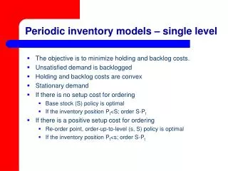
Periodic inventory models – single level
The objective is to minimize holding and backlog costs. Unsatisfied demand is backlogged Holding and backlog costs are convex Stationary demand If there is no setup cost for ordering Base stock (S) policy is optimal If the inventory position P t <S; order S-P t

Periodic inventory models – single level
E N D
Presentation Transcript
The objective is to minimize holding and backlog costs. Unsatisfied demand is backlogged Holding and backlog costs are convex Stationary demand If there is no setup cost for ordering Base stock (S) policy is optimal If the inventory position Pt<S; order S-Pt If there is a positive setup cost for ordering Re-order point, order-up-to-level (s, S) policy is optimal If the inventory position Pt<s; order S-Pt Periodic inventory models – single level
Ordering cost is for level i is the transportation cost from level i+1 to i Ordering cost for level n is the purchasing cost All ordering costs are linear, except at level n Backlog costs for level 1 is the backlog costs for external demand Backlog cost for level i is the cost of not being able to support level i-1 when level i-1 requested material Multi-echelon systems n n-1 2 1
Echelon stock for level 2 = on hand at level 2 + on hand at level 1 + on order from level 2 to level 1 Echelon inventory position for level 2 = echelon stock for level 2 + on order from level 3 to level 2 Similarly for level j If there is no setup cost for ordering Base stock (Sj) policy is optimal for each level j If the echelon inventory position Pjt<Sj; order Sj-Pjt If there is a positive setup cost for ordering Re-order point, order-up-to-level (sj, Sj) policy is optimal for each level j If the inventory position Pjt<sj; order Sj-Pjt Multi-echelon systems n n-1 2 1
Echelon stock for warehouse = on hand at retailer 1 + on hand at retailer 2 + on hand at warehouse + on hand at warehouse to retailers 1 & 2 Echelon inventory position for warehouse = echelon stock for warehouse on order from supplier to warehouse Assumption: no transshipments Assumption: retailer 1 and retailer 2 stocks are not seriously out of balance Base stock policy (S) for no setup case and (s, S) policy for setup case are optimal for the warehouse and retailers (using the echelon stock for warehouse) Tree like supply chains Supplier Warehouse Retailer 1 Retailer 2
Minimizing inventory subject to backorders • No repairs • Poisson demands at bases • Demand at depot l= l1+l2 • Re-order point at depot = S0 • Re-order point at bases S1,S2 • Expected number of units being delayed at the depot Supplier D Depot O2 O1 Base 1 Base 2 • Percentage delayed l1 l2
Minimizing inventory subject to backorders • Backorders at Base j Supplier D Depot O2 O1 • Problem Base 1 Base 2 l1 l2
Example • If the fill rate at the depot is 50% • Effective lead time at base 1 = 1+0.5*2=2 months • Effective lead time at base 2 = 2+0.5*2=3 months • If the fill rate at the depot is 75% • Effective lead time at base 1 = 1+0.25*2=1.5 months • Effective lead time at base 2 = 2+0.25*2=2.5 months • Effective lead time at the bases is a function of the depot fill rate, which is a function of stock level at the depot. • So fill rate at the base is a function of stock level at the base as well as stock level at the depot Supplier D=2 months Depot O2=2 months O1=1 month Base 1 Base 2 l1 l2
Managing inventory • ABC approach: Classify items into A, B, C classes. Tighter management of inventory for A items • Lead time reductions have major impact on inventories. • Inventory turnover ratio = (annual sales)/(average inventory level) • There is “economies of scale” in managing inventory. Fast moving items usually lead to larger inventory turns