Download
1 / 27
280 likes | 436 Vues
Flexible Energy Scheduling Tool for Integration of Variable generation. WECC VGS Operating Workgroup Salt Lake City Michael Milligan and Erik Ela Dec 7, 2011. Objective. VGS OWG is interested in assessing reserve methods, possibly recommending one or more

E N D
Flexible Energy Scheduling Tool for Integration of Variable generation WECC VGS Operating Workgroup Salt Lake City Michael Milligan and Erik Ela Dec 7, 2011
Objective • VGS OWG is interested in assessing reserve methods, possibly recommending one or more • Several methods have been proposed, but have not been rigorously tested • FESTIV model is a proposed platform (more later) • A few cases can be selected that represent alternative BA sizes/characteristics, and reserve approaches can be compared
Purpose of this presentation • Introduce the VGS OWG to FESTIV • Determine whether there is sufficient interest to • Conduct a more in-depth webinar on FESTIV • Move forward with reserve evaluation study using FESTIV
FESTIV • Flexible Energy Scheduling Tool for Integration of VG • SCUC, SCED, and AGC sub-models • Models at high resolution • Typically AGC, the highest resolution at 2-6 seconds • Models multiple time frames with communication between sub-models • Multiple chances of forecast error and forecast correction • Interval length, interval update frequency, and optimization horizon configurable
FESTIV • Flexible operating structures • Dispatch frequency, how reserves are used, stochastic vs. deterministic, AGC mode of operation, etc. • Deployment of operating reserves modeled • Contingency, load following, regulation, etc. • Reserves are held in one sub-model and used in another
FESTIV • Linear, dc power flow, with n-1 transmission contingencies (including phase shifters and HVDC) • AC power flow can be added if needed • no frequency response modeled, no hydro or CCGT modeling, no electrical losses • These can all be added (frequency response would be very large change, however.) • SCUC – MILP, SCED – LP, AGC – rule based
FESTIV • The model focuses on short-term reliability impacts (i.e. 1 day) • It can be used to compare inputs (e.g. VG penetrations) as well as scheduling strategies (e.g. dispatch frequency) • Metrics: • Extreme imbalances - CPS2 violations (with configurable L10 and CPS interval) • Total imbalances - Absolute ACE Energy (AACEE) • Variability of imbalances - sACE • Similar metrics can be made for line flow, voltage, etc. • e.g. Absolute Line Flow Exceedance in Energy (ALFEE)
FESTIV Flow Diagram Unit status and unit start-up for all units with start time > tRTCSTART Run DASCUC tRTC interval? no Data Flow yes Unit status and unit start-up for all units Run RTSCUC Process Flow t = t+tAGC tRTD interval? no yes Run RTSCED Dispatch schedules and reserve schedules for all units AGC schedule, realized generation for all units, production cost, and ACE Run AGC
DASCUC Model (GAMS) Minimize Production Costs Subject to • Piecewise linear cost curves • Start-up Costs • No-load Costs • Load Shedding Costs and Ancillary Services Penalty Costs • Storage Value (at end of day) • Generation equals Load • Ancillary Services are greater or equal to requirements • Transmission Flows are under limits • Including PTDF, or DC load flow options, including phase shifting transformer optimization • Generation min and max limits (wind limit is variable) • Commitment Constraints (e.g., min run, min down, max starts, must-run, etc.) • Ramp rates • Ancillary Services (with requirement set by user) • Regulation • Spin • Non-Spin • Replacement reserve (non-spin and spin) • Contingency Constraints • PTDF and LODF or DC load flow • Variable start-up cost dependent on off-line time • Storage optimization • Currently modeled after PHS, storage is in MWh
RTSCUC Model (GAMS) Minimize Production Costs Subject to • Piecewise linear cost curves • Start up Costs – QS Units only (QS with start times > TRTCSTART) • No Load Costs – QS Units only (QS with start times > TRTCSTART) • Load Shedding Costs and Ancillary Services Penalty Costs • Generation equals Load • Ancillary Services are greater or equal to requirements • Transmission Flows are under limits • Including PTDF including phase shifting transformer optimization • Generation min and max limits (wind limit is variable) • Commitment Constraints for QS Units (e.g., min run, min down, max starts, must-run, etc.) • Long start fixed from Day-Ahead • Ramp rates • Ancillary Services • Regulation • Spin • Non-Spin • Replacement reserve (non-spin and spin) • Contingency Constraints • PTDF and LODF
RTSCED Model (GAMS) Minimize Production Costs Subject to • Piecewise linear cost curves • Load Shedding Costs and Ancillary Services Penalty Costs • Generation equals Load • Ancillary Services are greater or equal to requirements • Transmission Flows are under limits • Including PTDF, or DC load flow options, including phase shifting transformer optimization • Generation min and max limits (wind limit is variable) • Ramp rates using actual data (discussed in future slide) • Ancillary Services • Regulation • Spin • Non-Spin • Replacement reserve (non-spin and spin) • Contingency Constraints • PTDF and LODF or DC load flow
AGC (Matlab) • 4 Types, run every (6 s) interval • Blind: Do not follow ACE, interpolate each dispatch schedule • Fast: Follow ACE each cycle • Smooth: Follow a ACE signal which is filtered and integrated (common procedure) • Lazy: A optimal compliance procedure • Based on Makarov et al “Value of Regulation Resources Based on Their Time Response” • Only use Regulation if it appears you are about to violate CPS2 • Units weighted based on ramp rates and only if given a regulation schedule in the prior SCED • Behavior Rates – A number between 0 and 1 on how well the unit follows its AGC signal
Reserve Pick ups (GAMS) • Identical to RTSCUC but has no regular frequency • How to trigger • Based on contingency occurring • Based on ACE > ACE threshold • Units that were on reserve can be used for dispatch • No regulation reserve requirements • Use emergency limits if available (generation and network) • Decide on what reserves get implemented • Spin vs. non-spin • After the RPU, reserve requirements will ramp up to full requirements within some time • Restoration period
Impact of Variability (Blind AGC) • Perfect forecasts
Impact of Uncertainty (Blind AGC) 5 minute SCED would have 288 SCED forecasts
Impact of AGC Operation (imbalance) 1:Blind 2:Fast 3:Smooth 4:Lazy
Impact of AGC Operation (Costs) 1:Blind 2:Fast 3:Smooth 4:Lazy