Download
1 / 16
162 likes | 418 Vues
Lossless Compression of Hyperspectral Images with Random Access Support. Wei Hsu Maya Khaneboubi Jonathan Solnit. Outline. What is a hyperspectral image? JPEG-7 and JPEG-LS Prediction CCAP Ordering Max Cut Partitioning Metrics Results Conclusion. What is a Hyperspectral Image?.

E N D
Lossless Compression of Hyperspectral Images with Random Access Support Wei Hsu Maya Khaneboubi Jonathan Solnit
Outline • What is a hyperspectral image? • JPEG-7 and JPEG-LS Prediction • CCAP • Ordering • Max Cut Partitioning • Metrics • Results • Conclusion
What is a Hyperspectral Image? • Spectral image sensors are used to get images of surfaces at several hundred different frequencies • Can detect minerals, soil types, water content • Represented as a 3D matrix 1.9908 MHz 2.2307 MHz 2.4790 MHz Image source: Cuprite - http://aviris.jpl.nasa.gov
JPEG-7 and JPEG-LS Prediction • JPEG-7: Chooses best of seven possible prediction schemes (three examples given below) • x(i,j) = x(i-1, j) = x(i-1, j-1) = (x(i,j-1) + x(i-1,j))/2 • JPEG-LS (simplified) • x(i,j) = min (x1, x2) if x3 = max(x1,x2,x3) = max (x1, x2) if x3 = min(x1,x2,x3) = x1 – x3 + x2 else
Correlation-based Conditional Average Prediction (CCAP)1 • Encode the first band using JPEG-LS • Encode subsequent bands depending on context matching • If ||xi – yi|| ≤ T y = (x/x1)y1 if x1 ≠ 0 = y1 else • Use JPEG-7 with the best predictor chosen by the previous band if context match not found Context in previous band Context in current band 1Wang, Babacan, Sayood 2005
CCAP Results • In addition to baseline CCAP, used JPEG-LS instead of JPEG-7 for band prediction if no context match found Scene images source: Foster, D.H., Nascimento, S.M.C., & Amano, K. 2004
Ordering • Ordering the bands can place highly correlated bands adjacent each other for better predictions • Model as a traveling salesman problem for a fully connected directed graph (shortest Hamiltonian path) • Edges are the entropies of the residuals between every pair of bands if compressed using CCAP
Bounded Prediction with Ordering for Random Access • Using prediction, decoding each band could require decoding the previous band • Worst case is having to decompress the entire hyperspectral image to see one band • Instead, can group the bands and only use prediction within that group • At most will have to download entire group, but less bands to predict from will result in less overall compression • Finding the optimal ordering with bounded prediction has been proven to be an NP-Hard problem2 2Tate 1997
Partitioning – Max Cut Algorithm • Similar graph model as for ordering, but undirected • Max cut partitions the graph by cutting the maximum sum of edge weights (average entropies) • Successive max cuts partition the bands into groups
Metrics • To evaluate performance, chose two metrics that illustrate the trade-off of bounded prediction • Bitrate per band – number of bits needed to download a single band • Expect a decrease with more groups • Normalized file size – used sum of entropies of bands to approximate file size • Expect an increase with more groups
Results – Bit Rate per Band (Scene7) Downsampled image for processing speed
Results – File Size (Scene7) Downsampled image for processing speed
Results – Bit Rate per Band (Cuprite) Downsampled image for processing speed
Results – File Size (Cuprite) Downsampled image for processing speed
Conclusion • Results varied depending on the image • Possible issues • Set threshold T empirically, should adapt to image • Edge weights in digraph don’t properly account for first band in group being encoded using JPEG-LS • Max cut as implemented takes the best single cut, not multiple cuts • Also required a symmetric adjacency matrix, had to average entropies