Introduction to Quantitative Analysis
Introduction to Quantitative Analysis. Chapter 1. Learning Objectives. After completing this chapter, students will be able to:. Describe the quantitative analysis approach Understand the application of quantitative analysis in a real situation


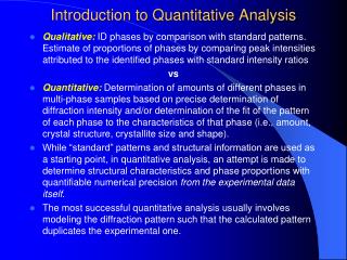
Introduction to Quantitative Analysis
E N D
Presentation Transcript
Introduction to Quantitative Analysis Chapter 1
Learning Objectives After completing this chapter, students will be able to: • Describe the quantitative analysis approach • Understand the application of quantitative analysis in a real situation • Describe the use of modeling in quantitative analysis • Discuss possible problems in using quantitative analysis • Perform a break-even analysis
Chapter Outline 1.1 Introduction 1.2 What Is Quantitative Analysis? 1.3 The Quantitative Analysis Approach 1.4 How to Develop a Quantitative Analysis Model 1.5 The Role of Computers and Spreadsheet Models in the Quantitative Analysis Approach 1.6 Possible Problems in the Quantitative Analysis Approach 1.7 Implementation — Not Just the Final Step
Introduction • Mathematical tools have been used for thousands of years • Quantitative analysis can be applied to a wide variety of problems • It’s not enough to just know the mathematics of a technique • One must understand the specific applicability of the technique, its limitations, and its assumptions
Examples of Quantitative Analyses • Taco Bell saved over $150 million using forecasting and scheduling quantitative analysis models • NBC television increased revenues by over $200 million by using quantitative analysis to develop better sales plans • Continental Airlines saved over $40 million using quantitative analysis models to quickly recover from weather delays and other disruption
Raw Data Quantitative Analysis Meaningful Information What is Quantitative Analysis? Quantitative analysis is a scientific approach to managerial decision making whereby raw data are processed and manipulated resulting in meaningful information
Scope of OR in Management • Marketing and sales – product selection and competitive strategies, utilization of salesman, their time and territory control, frequency of visits in sales force analysis, marketing advertising decision, forecasting, pricing and market research decision etc. • Production Management – product mix, maintenance policies, crew sizing and replacement system, project planning Quality Control decision and material handling facilities etc.
Purchasing, Procurement and Inventory Controls- buying policies levels, negotiations, bidding policies, time and quality of procurement. • Finance, Investment & Budgeting – Profit planning, cash flow analysis, investment policy for maximum return, dividend policies, investment decision , risk analysis and portfolio analysis etc.
What is Quantitative Analysis? Quantitative factorsmight be different investment alternatives, interest rates, inventory levels, demand, or labor cost Qualitative factorssuch as the weather, state and federal legislation, and technology breakthroughs should also be considered • Information may be difficult to quantify but can affect the decision-making process
Defining the Problem Developing a Model Acquiring Input Data Developing a Solution Testing the Solution Analyzing the Results Implementing the Results The Quantitative Analysis Approach Figure 1.1
Defining the Problem Need to develop a clear and concise statement that gives direction and meaning to the following steps • This may be the most important and difficult step • It is essential to go beyond symptoms and identify true causes • May be necessary to concentrate on only a few of the problems – selecting the right problems is very important • Specific and measurable objectives may have to be developed
Y = b0 + b1X $ Sales $ Advertising Schematic models Scale models Developing a Model Quantitative analysis models are realistic, solvable, and understandable mathematical representations of a situation There are different types of models
Developing a Model • Models generally contain variables (controllable and uncontrollable) and parameters • Controllable variables are generally the decision variables and are generally unknown • Parameters are known quantities that are a part of the problem
Garbage In Process Garbage Out Acquiring Input Data Input data must be accurate – GIGO rule Data may come from a variety of sources such as company reports, company documents, interviews, on-site direct measurement, or statistical sampling
Developing a Solution • The best (optimal) solution to a problem is found by manipulating the model variables until a solution is found that is practical and can be implemented • Common techniques are • Solving equations • Trial and error – trying various approaches and picking the best result • Complete enumeration – trying all possible values • Using an algorithm – a series of repeating steps to reach a solution
Testing the Solution Both input data and the model should be tested for accuracy before analysis and implementation • New data can be collected to test the model • Results should be logical, consistent, and represent the real situation
Analyzing the Results Determine the implications of the solution • Implementing results often requires change in an organization • The impact of actions or changes needs to be studied and understood before implementation Sensitivity analysis determines how much the results of the analysis will change if the model or input data changes • Sensitive models should be very thoroughly tested
Implementing the Results Implementation incorporates the solution into the company • Implementation can be very difficult • People can resist changes • Many quantitative analysis efforts have failed because a good, workable solution was not properly implemented Changes occur over time, so even successful implementations must be monitored to determine if modifications are necessary
Modeling in the Real World Quantitative analysis models are used extensively by real organizations to solve real problems • In the real world, quantitative analysis models can be complex, expensive, and difficult to sell • Following the steps in the process is an important component of success
How To Develop a Quantitative Analysis Model • An important part of the quantitative analysis approach • Let’s look at a simple mathematical model of profit Profit = Revenue – Expenses
How To Develop a Quantitative Analysis Model Expenses can be represented as the sum of fixed and variable costs and variable costs are the product of unit costs times the number of units Profit = Revenue – (Fixed cost + Variable cost) Profit = (Selling price per unit)(number of units sold) – [Fixed cost + (Variable costs per unit)(Number of units sold)] Profit = sX – [f+vX] Profit = sX – f –vX where s = selling price per unit v = variable cost per unit f = fixed cost X = number of units sold
The parameters of this model are f, v, and s as these are the inputs inherent in the model The decision variable of interest is X How To Develop a Quantitative Analysis Model Expenses can be represented as the sum of fixed and variable costs and variable costs are the product of unit costs times the number of units Profit = Revenue – (Fixed cost + Variable cost) Profit = (Selling price per unit)(number of units sold) – [Fixed cost + (Variable costs per unit)(Number of units sold)] Profit = sX – [f+vX] Profit = sX – f –vX where s = selling price per unit v = variable cost per unit f = fixed cost X = number of units sold
Pritchett’s Precious Time Pieces The company buys, sells, and repairs old clocks. Rebuilt springs sell for $10 per unit. Fixed cost of equipment to build springs is $1,000. Variable cost for spring material is $5 per unit. Profits = sX – f – vX s = 10 f = 1,000 v = 5 Number of spring sets sold = X If sales = 0, profits = –$1,000 If sales = 1,000, profits = [(10)(1,000) – 1,000 – (5)(1,000)] = $4,000
f s – v X = Fixed cost (Selling price per unit) – (Variable cost per unit) BEP = Pritchett’s Precious Time Pieces Companies are often interested in their break-even point (BEP). The BEP is the number of units sold that will result in $0 profit. 0 = sX – f – vX, or 0 = (s – v)X – f Solving for X, we have f = (s – v)X
BEP for Pritchett’s Precious Time Pieces BEP = $1,000/($10 – $5) = 200 units Sales of less than 200 units of rebuilt springs will result in a loss Sales of over 200 units of rebuilt springs will result in a profit f s – v X = Fixed cost (Selling price per unit) – (Variable cost per unit) BEP = Pritchett’s Precious Time Pieces Companies are often interested in their break-even point (BEP). The BEP is the number of units sold that will result in $0 profit. 0 = sX – f – vX, or 0 = (s – v)X – f Solving for X, we have f = (s – v)X
Models can accurately represent reality Models can help a decision maker formulate problems Models can give us insight and information Models can save time and money in decision making and problem solving A model may be the only way to solve large or complex problems in a timely fashion A model can be used to communicate problems and solutions to others Advantages of Mathematical Modeling
Objective Function – a mathematical expression that describes the problem’s objective, such as maximizing profit or minimizing cost Constraints – a set of restrictions or limitations, such as production capacities Uncontrollable Inputs – environmental factors that are not under the control of the decision maker Decision Variables – controllable inputs; decision alternatives specified by the decision maker, such as the number of units of Product X to produce Mathematical Models
The O’Neill Shoe Manufacturing company will produce a special-style shoe if the order size is large enough to provide a reasonable profit. For each special-style order, 5 hours are required to manufacture and only 40 hours of manufacturing time are available. The profit is $ 10 per pair. Let x denotes the number of pairs of shoes produced. Develop a mathematics model. Example : O’Neill Shoe Manufacturing company
The analyst attempts to identify the alternative (the set of decision variable values) that provides the “best” output for the model. The “best” output is the optimal solution. If the alternative does not satisfy all of the model constraints, it is rejected as being infeasible, regardless of the objective function value. If the alternative satisfies all of the model constraints, it is feasible and a candidate for the “best” solution Model Solution
One solution approach is trial-and-error. Might not provide the best solution Inefficient (numerous calculations required) Special solution procedures have been developed for specific mathematical models. Some small models/problems can be solved by hand calculations Most practical applications require using a computer Model Solution
Trial and Error Solution For The O’Neill Shoe Manufacturing Company
Iron Works, Inc. manufactures two products made from steel and just received this month's allocation of b pounds of steel. It takes a1 pounds of steel to make a unit of product 1 and a2 pounds of steel to make a unit of product 2. Let x1 and x2 denote this month's production level of product 1 and product 2, respectively. Denote by p1 and p2 the unit profits for products 1 and 2, respectively. Iron Works has a contract calling for at least m units of product 1 this month. The firm's facilities are such that at most u units of product 2 may be produced monthly. Example: Iron Works, Inc.
Mathematical Model The total monthly profit = (profit per unit of product 1) x (monthly production of product 1) + (profit per unit of product 2) x (monthly production of product 2) = p1x1 + p2x2 We want to maximize total monthly profit: Max p1x1 + p2x2 Example: Iron Works, Inc
Mathematical Model (continued) The total amount of steel used during monthly production equals: (steel required per unit of product 1) x (monthly production of product 1) + (steel required per unit of product 2) x (monthly production of product 2) = a1x1 + a2x2 This quantity must be less than or equal to the allocated b pounds of steel: a1x1 + a2x2 <b Example: Iron Works, Inc
Mathematical Model (continued) The monthly production level of product 1 must be greater than or equal to m : x1>m The monthly production level of product 2 must be less than or equal to u : x2<u However, the production level for product 2 cannot be negative: x2> 0 Example: Iron Works, Inc.
Mathematical Model Summary Max p1x1 + p2x2 s.t a1x1 + a2x2<b x1>m x2<u x2> 0 Example: Iron Works, Inc. Constraints Objective Function “Subject to”
Mathematical models that do not involve risk are called deterministic models We know all the values used in the model with complete certainty Mathematical models that involve risk, chance, or uncertainty are called probabilistic models Values used in the model are estimates based on probabilities Models Categorized by Risk
Possible Problems in the Quantitative Analysis Approach Defining the problem • Problems are not easily identified • Conflicting viewpoints • Impact on other departments • Beginning assumptions • Solution outdated Developing a model • Fitting the textbook models • Understanding the model
Possible Problems in the Quantitative Analysis Approach Acquiring input data • Using accounting data • Validity of data Developing a solution • Hard-to-understand mathematics • Only one answer is limiting Testing the solution Analyzing the results
Implementation – Not Just the Final Step Lack of commitment and resistance to change • Management may fear the use of formal analysis processes will reduce their decision-making power • Action-oriented managers may want “quick and dirty” techniques • Management support and user involvement are important
Implementation – Not Just the Final Step Lack of commitment by quantitative analysts • An analysts should be involved with the problem and care about the solution • Analysts should work with users and take their feelings into account
Summary • Quantitative analysis is a scientific approach to decision making • The approach includes • Defining the problem • Acquiring input data • Developing a solution • Testing the solution • Analyzing the results • Implementing the results
Summary • Potential problems include • Conflicting viewpoints • The impact on other departments • Beginning assumptions • Outdated solutions • Fitting textbook models • Understanding the model • Acquiring good input data • Hard-to-understand mathematics • Obtaining only one answer • Testing the solution • Analyzing the results
Summary • Implementation is not the final step • Problems can occur because of • Lack of commitment to the approach • Resistance to change