Relevance Feedback
Relevance Feedback. Main Idea: Modify existing query based on relevance judgements Extract terms from relevant documents and add them to the query and/or re-weight the terms already in the query Two main approaches: Automatic (psuedo-relevance feedback) Users select relevant documents

Relevance Feedback
E N D
Presentation Transcript
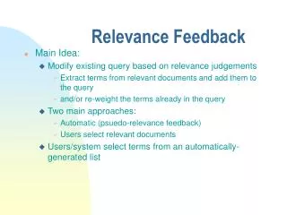
Relevance Feedback • Main Idea: • Modify existing query based on relevance judgements • Extract terms from relevant documents and add them to the query • and/or re-weight the terms already in the query • Two main approaches: • Automatic (psuedo-relevance feedback) • Users select relevant documents • Users/system select terms from an automatically-generated list
Relevance Feedback • Usually do both: • expand query with new terms • re-weight terms in query • There are many variations • usually positive weights for terms from relevant docs • sometimes negative weights for terms from non-relevant docs • Remove terms ONLY in non-relevant documents
Relevance Feedback for Vector Model In the “ideal” case where we know the relevant Documents a priori Cr = Set of documents that are truly relevant to Q N = Total number of documents
Rocchio Method Qo is initial query. Q1 is the query after one iteration Dr are the set of relevant docs Dn are the set of irrelevant docs Alpha =1; Beta=.75, Gamma=.25 typically. Other variations possible, but performance similar
Information 1.0 D1 Q’ 0.5 Q0 Q” D2 0 0.5 1.0 Retrieval Rocchio/Vector Illustration Q0 = retrieval of information = (0.7,0.3) D1 = information science = (0.2,0.8) D2 = retrieval systems = (0.9,0.1) Q’ = ½*Q0+ ½ * D1 = (0.45,0.55) Q” = ½*Q0+ ½ * D2 = (0.80,0.20)
Example Rocchio Calculation Relevant docs Non-rel doc Original Query Constants Rocchio Calculation Resulting feedback query
Rocchio Method • Rocchio automatically • re-weights terms • adds in new terms (from relevant docs) • have to be careful when using negative terms • Rocchio is not a machine learning algorithm • Most methods perform similarly • results heavily dependent on test collection • Machine learning methods are proving to work better than standard IR approaches like Rocchio
Relevance feedback in Probabilistic Model • sim(dj,q) ~ ~ wiq * wij * (log P(ki | R) + log P(ki | R) ) P(ki | R) P(ki | R) • Probabilities P(ki | R) and P(ki | R) ? • Estimates based on assumptions: • P(ki | R) = 0.5 • P(ki | R) = ni N where ni is the number of docs that contain ki • Use this initial guess to retrieve an initial ranking • Improve upon this initial ranking
Improving the Initial Ranking • sim(dj,q) ~ ~ wiq * wij * (log P(ki | R) + log P(ki | R) ) P(ki | R) P(ki | R) • Let • V : set of docs initially retrieved • Vi : subset of docs retrieved that contain ki • Reevaluate estimates: • P(ki | R) = Vi V • P(ki | R) = ni - Vi N - V • Repeat recursively Relevance Feedback..
Improving the Initial Ranking • sim(dj,q) ~ ~ wiq * wij * (log P(ki | R) + log P(ki | R) ) P(ki | R) P(ki | R) • To avoid problems with V=1 and Vi=0: • P(ki | R) = Vi + 0.5 V + 1 • P(ki | R) = ni - Vi + 0.5 N - V + 1 • Also, • P(ki | R) = Vi + ni/N V + 1 • P(ki | R) = ni - Vi + ni/N N - V + 1 Relevance Feedback..
Using Relevance Feedback • Known to improve results • in TREC-like conditions (no user involved) • What about with a user in the loop? • How might you measure this? • Precision/Recall figures for the unseen documents need to be computed
Relevance Feedback Summary • Iterative query modification can improve precision and recall for a standing query • In at least one study, users were able to make good choices by seeing which terms were suggested for R.F. and selecting among them
Query Expansion Add terms that are closely related to the query terms to improve precision and recall. Two variants: Local only analyze the closeness among the set of documents that are returned Global Consider all the documents in the corpus a priori How to decide closely related terms? THESAURI!! -- Hand-coded thesauri (Roget and his brothers) -- Automatically generated thesauri --Correlation based (association, nearness) --Similarity based (terms as vectors in doc space) --Statistical (clustering techniques)
Correlation/Co-occurrence analysis Co-occurrence analysis: • Terms that are related to terms in the original query may be added to the query. • Two terms are related if they have high co-occurrence in documents. Let n be the number of documents; n1 and n2 be # documents containing terms t1 and t2, m be the # documents having both t1 and t2 If t1 and t2 are independent If t1 and t2 are correlated Measure degree of correlation
Association Clusters • Let Mij be the term-document matrix • For the full corpus (Global) • For the docs in the set of initial results (local) • (also sometimes, stems are used instead of terms) • Correlation matrix C = MMT (term-doc Xdoc-term = term-term) Un-normalized Association Matrix Normalized Association Matrix Nth-Association Cluster for a term tu is the set of terms tv such that Suv are the n largest values among Su1, Su2,….Suk
Example 11 4 6 4 34 11 6 11 26 Correlation Matrix d1d2d3d4d5d6d7 K1 2 1 0 2 1 1 0 K2 0 0 1 0 2 2 5 K3 1 0 3 0 4 0 0 Normalized Correlation Matrix 1.0 0.097 0.193 0.097 1.0 0.224 0.193 0.224 1.0 1thAssoc Cluster for K2is K3
Scalar clusters Even if terms u and v have low correlations, they may be transitively correlated (e.g. a term w has high correlation with u and v). Consider the normalized association matrix S The “association vector” of term u Au is (Su1,Su2…Suk) To measure neighborhood-induced correlation between terms: Take the cosine-theta between the association vectors of terms u and v Nth-scalar Cluster for a term tu is the set of terms tv such that Suv are the n largest values among Su1, Su2,….Suk
Example Normalized Correlation Matrix AK1 USER(43): (neighborhood normatrix) 0: (COSINE-METRIC (1.0 0.09756097 0.19354838) (1.0 0.09756097 0.19354838)) 0: returned 1.0 0: (COSINE-METRIC (1.0 0.09756097 0.19354838) (0.09756097 1.0 0.2244898)) 0: returned 0.22647195 0: (COSINE-METRIC (1.0 0.09756097 0.19354838) (0.19354838 0.2244898 1.0)) 0: returned 0.38323623 0: (COSINE-METRIC (0.09756097 1.0 0.2244898) (1.0 0.09756097 0.19354838)) 0: returned 0.22647195 0: (COSINE-METRIC (0.09756097 1.0 0.2244898) (0.09756097 1.0 0.2244898)) 0: returned 1.0 0: (COSINE-METRIC (0.09756097 1.0 0.2244898) (0.19354838 0.2244898 1.0)) 0: returned 0.43570948 0: (COSINE-METRIC (0.19354838 0.2244898 1.0) (1.0 0.09756097 0.19354838)) 0: returned 0.38323623 0: (COSINE-METRIC (0.19354838 0.2244898 1.0) (0.09756097 1.0 0.2244898)) 0: returned 0.43570948 0: (COSINE-METRIC (0.19354838 0.2244898 1.0) (0.19354838 0.2244898 1.0)) 0: returned 1.0 Scalar (neighborhood) Cluster Matrix 1.0 0.226 0.383 0.226 1.0 0.435 0.383 0.435 1.0 1thScalar Cluster for K2is still K3
Metric Clusters average.. • Let r(ti,tj) be the minimum distance (in terms of number of separating words) between ti and tj in any single document (infinity if they never occur together in a document) • Define cluster matrix Suv= 1/r(ti,tj) Nth-metric Cluster for a term tu is the set of terms tv such that Suv are the n largest values among Su1, Su2,….Suk R(ti,tj) is also useful For proximity queries And phrase queries
Similarity Thesaurus • The similarity thesaurus is based on term to term relationships rather than on a matrix of co-occurrence. • obtained by considering that the terms are concepts in a concept space. • each term is indexed by the documents in which it appears. • Terms assume the original role of documents while documents are interpreted as indexing elements
Motivation Ki Kv Kj Ka Q Kb
Similarity Thesaurus • Terminology • t: number of terms in the collection • N: number of documents in the collection • Fi,j: frequency of occurrence of the term ki in the document dj • tj: vocabulary of document dj • itfj: inverse term frequency for document dj • Inverse term frequency for document dj • To ki is associated a vector Where Idea: It is no surprise if Oxford dictionary Mentions the word!
Similarity Thesaurus • The relationship between two terms ku and kv is computed as a correlation factor cu,v given by • The global similarity thesaurus is built through the computation of correlation factor Cu,v for each pair of indexing terms [ku,kv] in the collection • Expensive • Possible to do incremental updates… Similar to the scalar clusters Idea, but for the tf/itf weighting Defining the term vector
Query expansion with Global Thesaurus • three steps as follows: • Represent the query in the concept space used for representation of the index terms • Based on the global similarity thesaurus, compute a similarity sim(q,kv) between each term kv correlated to the query terms and the whole query q. • Expand the query with the top r ranked terms according to sim(q,kv)
Query Expansion - step one • To the query q is associated a vector q in the term-concept space given by where wi,q is a weight associated to the index-query pair[ki,q]
Query Expansion - step two • Compute a similarity sim(q,kv) between each term kv and the user query q • where Cu,v is the correlation factor
Query Expansion - step three • Add the top r ranked terms according to sim(q,kv) to the original query q to form the expanded query q’ • To each expansion term kv in the query q’ is assigned a weight wv,q’ given by • The expanded query q’ is then used to retrieve new documents to the user
Statistical Thesaurus formulation • Expansion terms must be low frequency terms • However, it is difficult to cluster low frequency terms • Idea: Cluster documents into classes instead and use the low frequency terms in these documents to define our thesaurus classes. • This algorithm must produce small and tight clusters.
A clustering algorithm (Complete Link) • This is document clustering algorithm with produces small and tight clusters • Place each document in a distinct cluster. • Compute the similarity between all pairs of clusters. • Determine the pair of clusters [Cu,Cv] with the highest inter-cluster similarity. • Merge the clusters Cu and Cv • Verify a stop criterion. If this criterion is not met then go back to step 2. • Return a hierarchy of clusters. • Similarity between two clusters is defined as the minimum of similarities between all pair of inter-cluster documents
Selecting the terms that compose each class • Given the document cluster hierarchy for the whole collection, the terms that compose each class of the global thesaurus are selected as follows • Obtain from the user three parameters • TC: Threshold class • NDC: Number of documents in class • MIDF: Minimum inverse document frequency
Selecting the terms that compose each class • Use the parameter TC as threshold value for determining the document clusters that will be used to generate thesaurus classes • This threshold has to be surpassed by sim(Cu,Cv) if the documents in the clusters Cu and Cv are to be selected as sources of terms for a thesaurus class • Use the parameter NDC as a limit on the size of clusters (number of documents) to be considered. • A low value of NDC might restrict the selection to the smaller cluster Cu+v
Selecting the terms that compose each class • Consider the set of document in each document cluster pre-selected above. • Only the lower frequency documents are used as sources of terms for the thesaurus classes • The parameter MIDF defines the minimum value of inverse document frequency for any term which is selected to participate in a thesaurus class
Query Expansion based on a Statistical Thesaurus • Use the thesaurus class to query expansion. • Compute an average term weight wtc for each thesaurus class C
Query Expansion based on a Statistical Thesaurus • wtc can be used to compute a thesaurus class weight wc as
Query Expansion Sample Doc1 = D, D, A, B, C, A, B, C Doc2 = E, C, E, A, A, D Doc3 = D, C, B, B, D, A, B, C, A Doc4 = A q= A E E • TC = 0.90 NDC = 2.00 MIDF = 0.2 sim(1,3) = 0.99 sim(1,2) = 0.40 sim(1,2) = 0.40 sim(2,3) = 0.29 sim(4,1) = 0.00 sim(4,2) = 0.00 sim(4,3) = 0.00 idf A = 0.0 idf B = 0.3 idf C = 0.12 idf D = 0.12 idf E = 0.60 q'=A B E E
Query Expansion based on a Statistical Thesaurus • Problems with this approach • initialization of parameters TC,NDC and MIDF • TC depends on the collection • Inspection of the cluster hierarchy is almost always necessary for assisting with the setting of TC. • A high value of TC might yield classes with too few terms
Conclusion • Thesaurus is a efficient method to expand queries • The computation is expensive but it is executed only once • Query expansion based on similarity thesaurus may use high term frequency to expand the query • Query expansion based on statistical thesaurus need well defined parameters
Using correlation for term change • Low freq to Medium Freq • By synonym recognition • High to medium frequency • By phrase recognition

