Suffix Trees
Suffix Trees. Outline. Introduction Suffix Trees (ST) Building STs in linear time: Ukkonen’s algorithm Applications of ST. Introduction. Substrings. String is any sequence of characters. Substring of string S is a string composed of characters i through j , i j of S .


Suffix Trees
E N D
Presentation Transcript
Outline • Introduction • Suffix Trees (ST) • Building STs in linear time: Ukkonen’s algorithm • Applications of ST
Substrings • String is any sequence of characters. • Substring of string S is a string composed of characters i through j, ij of S. • S = cater;ate is a substring. • car is not a substring. • Empty string is a substring of S.
Subsequences • Subsequence of string S is a string composed of characters i1 < i2 < … < ik of S. • S = cater; ate is a subsequence. • car is a subsequence. • Empty string is a subsequence of S.
String/Pattern Matching - I • You are given a source string S. • Suppose we have to answer queries of the form: is the string pia substring of S? • Knuth-Morris-Pratt (KMP) string matching. • O(|S| + | pi |) time per query. • O(n|S| + Si | pi |) time for n queries. • Suffix tree solution. • O(|S| + Si | pi |) time for n queries.
String/Pattern Matching - II • KMP preprocesses the query string pi, whereas the suffix tree method preprocesses the source string (text) S. • The suffix tree for the text is built in O(m) time during a pre-processing stage; thereafter, whenever a string of length O(n) is input, the algorithm searches it in O(n) time using that suffix tree.
String Matching: Prefixes & Suffixes • Substrings of S beginning at the first position of S are called prefixes of S, and substrings that end at its last position are called suffixes of S. • S=AACTAG • Prefixes: AACTAG,AACTA,AACT,AAC,AA,A • Suffixes: AACTAG,ACTAG,CTAG,TAG,AG,G • pi isa substring of S iff pi isa prefix of some suffix of S.
Definition:Suffix Tree (ST) T for S of length m 1. A rooted treewith mleaves numbered from 1 to m. 2. Each internal node, excluding the root, of Thas atleast 2 children. 3. Each edge of Tis labeled with a nonemptysubstring of S. 4. No two edges out of a node can have edge-labelsstarting with the same character. 5. For any leaf i, the concatenation ofthe edge-labels on the path from the root to leaf i exactly spells out the suffix of S, namely S[i,m], that starts at position i.
Existence of a suffix tree S • If one suffix Sjof Smatches a prefix of anothersuffix Siof S, then the path for Sjwould not endat a leaf. • S= xabxa • S1 = xabxa and S4 = xa • How to avoid this problem? • Assume that the last character of S appearsnowhere else in S. • Add a new character $ not in the alphabet tothe end of S.
Building STs in linear time: Ukkonen’s algorithm
Building STs in linear time • Weiner’s algorithm [FOCS, 1973] • ”The algorithm of 1973” called by Knuth • First algorithm of linear time, but much space • McGreight’s algorithm [JACM, 1976] • Linear time and quadratic space • More readable • Ukkonen’s algorithm [Algorithmica, 1995] • Linear time algorithm and less space • This is what we will focus on
Implicit Suffix Trees • Ukkonen’s algorithm constructs a sequence of implicit STs, the last of which is converted to a true ST of the given string. • An implicit suffix tree for string S is a tree obtained from the suffix tree for S$ by • removing $ from all edge labels • removing any edges that now have no label • removing any node that does not still have at least two children • An implicit suffix tree for prefix S[1,i] of S is similarly defined based on the suffix tree for S[1,i]$. • Ii will denote the implicit suffix tree for S[1,i]. • Each suffix is in the tree, but may not end at a leaf.
Example: Construction of theImplicit ST • Implicit tree for xabxa from tree for xabxa$ • {xabxa$, abxa$, bxa$, xa$, a$, $} b x a $ x a 6 a $ b $ x 5 b $ x a a 4 $ $ 3 2 1
Construction of the Implicit ST:Remove $ • Remove $ • {xabxa$, abxa$, bxa$, xa$, a$, $} b x a $ x a 6 a $ b $ x 5 b $ x a a 4 $ $ 3 2 1
Construction of the Implicit ST: After the Removal of $ • Remove $ • {xabxa, abxa, bxa, xa, a} b x a x a 6 a b x 5 b x a a 4 3 2 1
Construction of the Implicit ST: Remove unlabeled edges • Remove unlabeled edges • {xabxa, abxa, bxa, xa, a} b x a x a 6 a b x 5 b x a a 4 3 2 1
Construction of the Implicit ST: After the Removal of Unlabeled Edges • Remove unlabeled edges • {xabxa, abxa, bxa, xa, a} b x a x a a b x b x a a 3 2 1
Construction of the Implicit ST: Remove interior nodes • Remove internal nodes with only one child • {xabxa, abxa, bxa, xa, a} b x a x a a b x b x a a 3 2 1
Construction of the Implicit ST: Final implicit tree • Remove internal nodes with only one child • {xabxa, abxa, bxa, xa, a} b x x a a a b b x x a a 3 2 1
Ukkonen’s Algorithm (UA) • Ii is the implicit suffix tree of the string S[1, i] • Construct I1 • /* Construct Ii+1from Ii */ • for i = 1 to m-1 do /* phase i+1 */ • for j = 1 to i+1 do /* extension j */ • Find the end of the path Pfrom the root whose label is S[j, i]in Ii and extend Pwith S[i+1]by suffix extension rules; • Convert Im into a suffix tree S
Example • S = xabxacd$ • i+1 = 1 • x • i+1 = 2 • extend x to xa • a • i+1 = 3 • extend xa to xab • extend a to ab • b • …
Extension Rules • Goal: extend each S[j,i] into S[j,i+1] • Rule 1:S[j,i] ends at a leaf • Add character S(i+1) to the end of the label on that leaf edge • Rule 2:S[j,i] doesn’t end at a leaf, and the following character is not S(i+1) • Split a new leaf edge for character S(i+1) • May need to create an internal node if S[j,i] ends in the middle of an edge • Rule 3:S[j,i+1] is already in the tree • No update
a b x x x b a b a b b x 4 b x b 5 b x 3 b 2 1 Example: Extension Rules • Implicit tree for axabxb from tree for axabx b Rule 1: at a leaf node Rule 2: add a leaf edge (and an interior node) Rule 3: already in tree
S[1,3]=axa E S(j,i) S(i+1) 1 ax a 2 x a 3 a UA for axabxc (1)
Observations • Once S[j,i] is located in the tree, extension rules take only constant time • Naively we could find the end of any suffix S[j,i] in O(S[j,i])timeby walking from the root of the current tree. By that approach, Imcould be created in O(m3) time. • Making Ukkonen’s algorithm O(m) • Suffix links • Skip and count trick • Edge-label compression • A stopper • Once a leaf, always a leaf
Suffix Links • Consider the two strings aand xa • Suppose some internal node v of the tree is labeled with xa and another node s(v) in the tree is labeled with a • The edge (v,s(v)) is called a suffix link • Do all internal nodes (the root is not considered an internal node) have suffix links?
$ AC C $ AC $ AC $ AC $ AC AC$ $ $ AC$ Example:suffix links S = ACACACAC$
Suffix Link Lemma • If a new internal node v with path-label xa is added to the current tree in extensionj of some phase i+1, then • the path labeled a already ends at an internal node of the tree or • the internal node labeled a will be created in the extension of j+1 in the same phase i+1 • string a is empty and s(v) is the root
Proof of Suffix Link Lemma • A new internal node is created only by the extension rule 2 • This means that there are two distinct suffixes of S[1,i+1] that start with xa • xaS(i+1) and xacb where c is not S(i+1) • This means that there are two distinct suffixes of S[1,i+1] that start with a • aS(i+1) and acb where c is not S(i+1) • Thus, if a is not empty, a will label an internal node once extension j+1 is processed which is the extension of a
Corollary of Suffix Link Lemma • Every internal node of an implicit suffix tree has asuffix link from it.
How to use suffix links - 1 • S[1,i] must end at a leaf since it is the longest string in the implicit tree Ii • Keep a pointer to this leaf in all cases and extend according to rule 1 • Locating S[j+1,i] from S[j,i] which is at node w • If w is an internal node, set v to w • Otherwise, set v = parent(w) • If v is the root, you must traverse from the root to find S[j+1,i] • If not, go to s(v) and begin search for the remaining portion of S[j,i] from there
Skip and Count Trick – (1) • Problem: Moving down from s(v), directly implemented, takes time proportional to the number of characters compared • Solution: To makerunning time proportional to the number of nodes in the path searched, instead of the number of characters
Skip and Count Trick – (2) • After 4 nodes down-skips, the end of S[j, i]isfound.
Skip and Count Trick – (3) • Node-depth of v, denoted (ND(v)), is the number of nodes on the path from the root to the node v • Lemma: For any suffix link (v, s(v)) traversed in Ukkonen’s algorithm, at that moment, ND(v) ND(s(v))+1
Skip and Count Trick – (4) • At the moment of traversing (v,s(v)): ND(v) ND(s(v))+1
Skip and Count Trick – (5) • The current node-depth of the algorithm is the node depth of the node most recently visited by the algorithm • Lemma:Using the skip and count trick, any phase of Ukkonen’salgorithm takes O(m)time. • Up-walk: decreases the current node-depth by 1 • Suffix link traversal: same as up-walk • Totally, the current node-depth is decreased by2m. • No node has depth >m. • The total possible increment to the currentnode-depth is 3m.
Edge Label Representation • Potential Problem • Size of edge labels may require W(m2) space • Thus, the time for the algorithm is at least as large as the size of its output • Example • S = abcdefghijklmnopqrstuvwxyz • Total length is Sj<m+1j = m(m+1)/2 • Similar problem can happen when the length of the string is arbitrarily larger than the alphabet size • Solution • Label edges with pair of indices indicating beginning and end of positions of the substring in S
Modified Extension Rules • Rule 2: new leaf edge (phase i+1) • create edge (i+1, i+1) • split edge (p, q) => (p, w) and (w + 1, q) • Rule 1: leaf edge extension • label had to be (p,i) before extension • given rule 2 above and an induction argument: • (p, q) => (p, q + 1) • Rule 3 • Do nothing
Full edge label representation • String S = xabxa$ b x a $ x a 6 a $ b $ x 5 b $ x a a 4 $ $ 3 2 1
Edge-label Compression • String S = xabxa$ (1,2) [or (4,5)?] (2,2) (6,6) (3,6) 6 (6,6) 5 (6,6) (3,6) (3,6) 4 3 2 1
A Stopper • In any phase, if suffix extension rule 3 applies inextension j, it will also apply in all extensions k,where k>j, until the end of the phase. • The extensions in phase i+1 that are done after the first execution of rule 3 are said to be done implicitly. This is in contrast to any extension j where the end of S[j, i]is explicitly found. An extension of that kind is called and explicit extension. • Hence, we can end any phase i+1when the firstextension rule 3 applies.
Once a leaf, always a leaf – (1) • If at some point in UA a leaf is created and labeled j (for the suffix starting at position j of S), then that leaf will remain a leaf in all successive trees created during the algorithm. • In any phase i, there is an initial sequence ofconsecutive extensions (starting with extension 1) inwhich only rule 1 or 2 applies, where let jibe thelast extension in this sequence. • Note that jiji+1.