Download
1 / 33
330 likes | 520 Vues
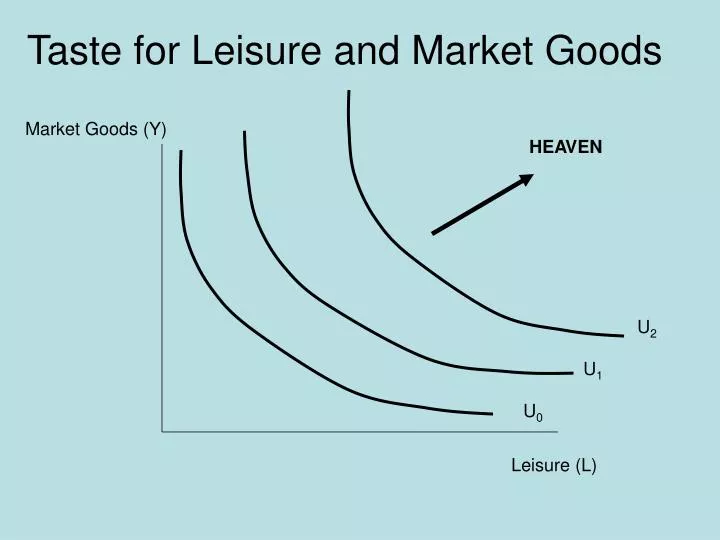
Taste for Leisure and Market Goods. Market Goods (Y). HEAVEN. U 2. U 1. U 0. Leisure (L). Budget Constraint for Leisure and Market Goods. Y = W(T – FT – L)+ Y N W = 5 = real wage T=24 FT=10 Y N =0 Y = 5H. Market Goods (Y). infeasible. 70. Slope = -W = -5. feasible. 0. 14.

E N D
Taste for Leisure and Market Goods Market Goods (Y) HEAVEN U2 U1 U0 Leisure (L)
Budget Constraint for Leisure and Market Goods Y = W(T – FT – L)+ YN W = 5 = real wage T=24 FT=10 YN =0 Y = 5H Market Goods (Y) infeasible 70 Slope = -W = -5 feasible 0 14 Leisure (L) 14 0 Hours of work (H)
Budget Constraint for Leisure and Market Goods Y = W(T – FT – L) + YN Wage rises to $6 Y = 6H Market Goods (Y) Income increase 70 Slope = -W = -6, so price of leisure increases Slope = -W = -5 0 14 Leisure (L) 14 0 Hours of work (H)
Budget Constraint for Leisure and Market Goods Y = W(T – FT – L) + YN Nonlabor income rises to YN = 20 Y = 5H + 20 Market Goods (Y) 90 Income increase 70 Slope = -W = -5 0 14 Leisure (L) 14 0 Hours of work (H)
Taste for Leisure and Market Goods Market Goods (Y) HEAVEN A W = (MUL / MUY) B U2 U1 U0 C Leisure (L)
Taste for Leisure and Market Goods Market Goods (Y) A W < (MUL / MUY) W = (MUL / MUY) B U2 U1 U0 C W > (MUL / MUY) Leisure (L)
Taste for Leisure and Market Goods Market Goods (Y) Who has the stronger taste for Leisure? Y0 UA Y1 UB L0 LB LA Leisure (L)
Taste for Leisure and Market Goods Market Goods (Y) Flatter indifference curve means Goods lover A YA UA Steeper indifference curve means Leisure lover B YB UB LA LB Leisure (L)
Work and Leisure: First-Year College Students National Survey of Student Engagement, 2000 data
Two simultaneous effects of a wage change Income effect: Change in leisure demand caused by a change in income, holding the wage rate constant If leisure is a normal good, an increase in income increase leisure demand and lowers labor supply. Substitution effect: Change in leisure demand caused by change in wage rate, holding utility constant. An increase in wage lowers leisure demand
Response to a wage increase Income effect toward goods toward leisure (away from hours of work) Substitution effect toward goods away from leisure (toward hours of work) Total toward goods leisure demand (labor supply) ambiguous
Response to a wage increase Income effect toward goods toward leisure (away from hours of work) Substitution effect toward goods away from leisure (toward hours of work) Total toward goods toward leisure demand (away from labor supply) Backward-bending labor supply: If income effect dominates substitution effect, a wage increase lowers labor supply
Response to a wage increase Income effect toward goods toward leisure (away from hours of work) Substitution effect toward goods away from leisure (toward hours of work) Total toward goods toward leisure demand (away from labor supply) Upward-sloping labor supply: If substitution effect dominates income effect, a wage increase raises labor supply
Effect depends on what happens to the budget constraint Change in slope =>substitution effect steeper=> wage increase flatter => wage decrease Change in height => income effect higher => income increasing lower => income falling
Empirical estimates Hours = a0 + a1*Wage + a2*Nonlabor Income +… Income effect = a2; Substitution effect derived from a1 and a2 Effect of 10% wage increase on labor supply Male Female Income effect -2% -1% Substitution effect 2% 4% Total effect -0% 3%
Empirical estimates Hours = a0 + a1*Wage + a2*Nonlabor Income +… Income effect = a2; Substitution effect derived from a1 and a2 Effect of 10% wage increase on labor supply Male Female Income effect -2% -1% Substitution effect 2% 4% Total effect -0% 3% “Backward- Bending” Labor Supply “Upward Sloping” Labor Supply
Why would wage increases have an particularly large effect on women?
Why does divorce raise labor supply for women ?and lower labor supply for men? Marital Status Male Female Single (never married) 70.2 65.9 Married (spouse present) 77.1 60.5 Divorced 73.5 71.5 Labor Force Participation Rates, by Gender, Marital Status, 2004 Bureau of Labor Statistics: http://www.bls.gov/cps/wlf-table4-2005.pdf
Social Security Retirement Earnings Test Applies to retirees between 62 and 65* *Normal retirement age rising to 66 by 2009 to 67 by 2027 For workers below normal retirement age, get full benefits if earnings below exempt amount Benefits fall $0.50 for every $ earned beyond the exempt amount until benefits go to zero
Social Security Annual Retirement Earnings Test Exempt Amounts, Ages below Normal Retirement Age ---------------------------------------------------------------------- Year Exempt income 2000 $10,080 2001 $10,680 2002 $11,280 2003 $11,520 2004 $11,640 2005 $12,000 2006 $12,480
48% of retired persons have no pension income except Social Security GAO. 2000. Characteristics of Persons without Pension Coverage in the Labor Force http://www.gao.gov/archive/2000/he00131.pdf
2/3 of retired women have no pension income except Social Security GAO. 2000. Characteristics of Persons without Pension Coverage in the Labor Force http://www.gao.gov/archive/2000/he00131.pdf
Iowa Unemployment Insurance Replacement rate: Percent of previous earnings that are replaced by benefit Typical is ~50% Why is replacement rate < 100%? Why is benefit conditional on being laid off or quitting for cause?
Iowa Unemployment Insurance In 1984, Iowa’s UI program was $304 million in the red. Interest on debt $1 million per month Proposal—continue to pay partial benefits after UI recipient finds work
As of 2004, Iowa UI fund was $683 million surplus 2004 Status Report On The Unemployment Insurance Trust Fund
Iowa Unemployment Insurance Benefit tied to previous earnings (highest quarter of previous four excluding the current and once lagged quarter) Average weekly wage = $586 If 0 dependents, 53% of previous earnings up to $310/week 4+ dependents: 65% of previous earnings up to $381/week You can earn up to 25% of weekly benefit in earnings and still get full benefit. After that, earnings taxed at 100% until benefit is exhausted 2004 Status Report On The Unemployment Insurance Trust Fund
Iowa Unemployment Insurance Example Wage = $14.65/hour ($586 per week) UI Benefit = 65% of previous earnings = $380 25% of benefit = $95 = max allowable labor earnings Possible part-time job = $9.50/hour 2004 Status Report On The Unemployment Insurance Trust Fund
Value of time and Labor Force Participation2003 dollars ChildrenService Price(1)Opportunity Cost(2) Ages <6 $27,736 $24,632 Ages 6-14 $24,960 $21,259 None $20,133 $19,997 (1) Over estimate (2) Under estimate