Compound Data Structures
Explore structural decomposition, arrays, linear vectors, multidimensional arrays, array access operations, and type declarations. Learn about the semantics of type declarations and storage allocation strategies. Discover innovative techniques for manipulating arrays efficiently in programming languages.

Compound Data Structures
E N D
Presentation Transcript
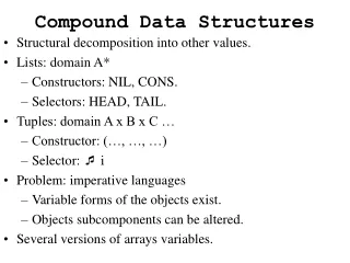
Compound Data Structures • Structural decomposition into other values. • Lists: domain A* • Constructors: NIL, CONS. • Selectors: HEAD, TAIL. • Tuples: domain A x B x C … • Constructor: (…, …, …) • Selector: i • Problem: imperative languages • Variable forms of the objects exist. • Objects subcomponents can be altered. • Several versions of arrays variables.
Arrays • Collection of homogeneous objects indexed by a set of scalar values. • Homogeneity all components have same structure. • Allocation of storage and typechecking easy. • Both tasks can be performed by compiler. • Selector operation: indexing. • Scalar index set: primitive domain with relational and arithmetic operations. • Restricted by lower and upper bounds.
Linear Vector of Values • IDArray = (Index Location) x Lowerbound x UpperBound • Index is index set • lessthan, greaterthan, equals. • Lowerbound = Upperbound = Index. • First component maps indices to the locations that contain the storable values. • Second and third component denote the bounds allowed on array indices.
Multidimensional Arrays • Array may contain other arrays. • Threedimensional array is vector whose components are twodimensional vectors. • Hierarchy of arrays defined as infinite sum • 1DArray = (Index Location) x Index x Index. • (n+1)DArray = (Index nDArray) x Index x Index. • 1DArray maps indices to locations, 2DArray maps indices to 1D arrays, . . . .
Multidimensional Arrays • a MDArray = inkDArray(map, lower, upper) for some k >= 1 • accessarray: Index MDArray (Location + MDArray + Errvalue) • accessarray = i. r. cases r of is1DArray(a) index1 a i [] is2DArray(a) index2 a i . . . [] iskDArray(a) indexK a i . . . end
index m = (map, lower, upper). i. (i lessthan lower) or (i greaterthan upper) inErrvalue() [] MInject(map(i)) 1Inject = l.inLocation(l) . . . (n+1)Inject = a. inMDArray( innDArray(a))
Multidimensional Arrays • accessarray is represented by an infinite function expression. • By using pair representation of disjoint union elements, operation is convertible to finite, computable format. • Operation performs onelevel indexing upon array a returning another array if a has more than one dimension. • Still model is to clumsy to be used in practice. • Real programming languages allow arrays of numbers, record structures, sets, . . . !
System of Type Declarations T Typestructure S Subscript T ::= nat| bool| array [N1... N2] of T |record D end D ::= D1;D2|var I:T C ::= …| I[S]:= E |... E ::= ... | I[S] |... S ::= E | E, S
Denotablevalue = (Natlocn + Boollocn + Array + Record + Errvalue) l Natlocn = Boollocn = Location a Array = (Nat Denotablevalue) x Nat x Nat r Record = Environment = Id Denotablevalue
Semantics of Type Declarations • T: Typestructure Store (Denotablevalue x Poststore) • T[[nat]] = s: let (l,p) = (allocatelocn s) in (inNatlocn(l), p) • T[[bool]] = s: let (l,p) = (allocatelocn s) in (inBoollocn(l), p)
T[[array [N1... N2]of T]] = s: let n1 = N[[N1]] in let n2 = N[[N2]] in n1 greaterthan n2 (inErrvalue(), (signalerr s)) [] getstorage n1 (emptyarray n1 n2 ) s • T[[record D end]] = s: let (e, p) = (D[[D]] emptyenv s) in (inRecord(e), p) Type structure expressions are mapped to storage allocation actions!
Semantics of Type Declarations • getstorage: Nat Array Store (Denotablevalue x Poststore) • getstorage = n: a: s: n greater n 2 (inArray(a), return s) [] let (d, p) = T[[T]]s in (check(getstorage (n plus one) (augmentarray n d a)))(p)
augmentarray: Nat Denotablevalue Array Array • augmentarray = n: d: (map, lower, upper): ([n | d] map, lower, upper) • emptyarray: Nat Nat Array • emptyarray = n1 : n2 :(( n:inErrvalue()); n1 ; n2 ) • getstorage iterates from lower bound of array to upper bound allocating the proper amount of storage for a component. • augmentarray inserts the component into the array.
Declarations • D: Declaration Environment Store (Environment x Poststore) • D[[D1;D2 ]] = e: s: let (e’, p’) = (D[[D1]]e s) in (check (D[[D2 ]]e’))(p) • D[[var I:T]] = e: s: let (d, p) = T[[T]]s in ((updateenv [[I]] d e), p) • A declaration activates the storage allocation strategy specified by its type structure.
Array Indexing S: Subscript Array Environment Store Storablevalue S[[E]] = a:e: s: cases (E[[E]]e s) of . . . [] isNat(n) accessarray n a … end S[[E, S]] = a: e: s: cases (E[[E]]e s) of … [] isNat(n) (cases (accessarray n a) of … [] isArray(a’ ) S[[S]]a’ e s ...end) ... end
Array Assignment C[[I[S] := E]] = e: s: cases (accessenv [[I]] e) of ... [] isArray(a) (cases (S[[S]]a e s) of ... isNatlocn(l) (cases (E[[E]]e s) of ... [] isNat(n) return(update l inNat(n) s) ...end) ...end) ...end Assignment is first order (location, not an array, is on lefthandside).