Download
1 / 85
870 likes | 1k Vues
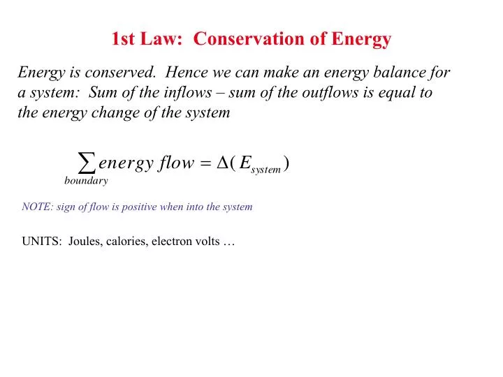
1st Law: Conservation of Energy. Energy is conserved. Hence we can make an energy balance for a system: Sum of the inflows – sum of the outflows is equal to the energy change of the system. NOTE: sign of flow is positive when into the system. UNITS: Joules, calories, electron volts ….

E N D
1st Law: Conservation of Energy Energy is conserved. Hence we can make an energy balance for a system: Sum of the inflows – sum of the outflows is equal to the energy change of the system NOTE: sign of flow is positive when into the system UNITS: Joules, calories, electron volts …
Types of Work Electrical W = – dq Magnetic Surface W = – dA
Variables and Parameters System is only described by its macroscopic variables Variables:Temperature + one variable for every work term that exchanges energy with the system + one variable for every independent component that can leave or enter the system. Parameters: Quantities that are necessary to describe the system but which do not change as the system undergoes changes. e.g. for a closed system: ni are parameters for a system at constant volume: V is parameter Equations of State (Constitutive Relations): equation between the variables of the system. One for each work term or matter flow
Example of Equations of State • pV = nRT: for ideal gas • = E efor uniaxial elastic deformation M = H: paramagnetic material
Properties and State Functions U = U(variables) e.g. U(T,p) for simple system Heat capacity Volumetric thermal expansion Compressibility
Some Properties Specific to ideal gasses ONLY for IDEAL GASSES • PV = nRT 2) cp - cv = R 3) Proof that for ideal gas, internal energy only depends on temperature
The Enthalpy (H) H = U + PV Gives the heat flow for any change of a simple system that occurs under constant pressure Example: chemical reaction
Enthalpy of Materials is always relative Elements: set to zero in their stable state at 298K and 1 atm pressure Compounds: tabulated. Are obtained experimentally by measuring the heat of formation of the compounds from the elements under constant pressure.
Entropy and the Second Law There exists a Property of systems, called the Entropy (S), for which holds: How does this solve our problem ?
The Second Law leads to Evolution Laws Isolated system
Evolution Law for constant Temperature and Pressure dG ≤ 0 G (Gibbs free energy is the relevant potential to determine stability of a material under constant pressure and temperature
Interpretation For purely mechanical systems: Evolution towards minimal energy. Why is this not the case for materials ? Materials at constant pressure and temperature can exchange energy with the environment. G is the most important quantity in Materials Science determines structure, phase transformation between them, morphology, mixing, etc.
Phase Diagrams: One component Describes stable phase (the one with lowest Gibbs free energy) as function of temperature and pressure. Water Carbon
What is a solution ? SYSTEM with multiple chemical components that is mixed homogeneously at the atomic scale • Liquid solutions • Vapor solutions • Solid Solutions
Composition Variables MOLE FRACTION: ATOMIC PERCENT: CONCENTRATION: WEIGHT FRACTION:
Variables to describe Solutions G=G(T,p,n1,n2, …, nN) Partial Molar Quantity Partial Molar Quantity chemical potential
Partial molar quantities give the contribution of a component to a property of the solution
Properties of Mixing Change in reaction: XA A + XB B -> (XA,XB )
Cu-Pd Ni-Pt
General Equilibrium Condition in Solutions Chemical potential for a component has to be the same in all phases For all components i OPEN SYSTEM Components have to have the same chemical potential in system as in environment e.g. vapor pressure
Summary so far 1) Composition variables 2) Partial Molar Quantities 3) Quantities for mixing reaction 4) Relation between 2) and 3): Intercept rule 5) Equilibrium between Solution Phases
Standard State: Formalism for Chemical Potentials in Solutions chemical potential of i in solution effect of concentration chemical potential of i in a standard state Choice of standard state is arbitrary, but often it is taken as pure state in same phase. Choice affects value of ai
Models for Solution: Ideal Solution An ideal solution is one in which all components behave Raoultian
Solutions: Homogeneous at the atomic level Ordered solutions Random solutions
Summary so far 1) Composition variables 2) Partial Molar Quantities 3) Quantities for mixing reaction 4) Relation between 2) and 3): Intercept rule 5) Equilibrium between components in Solution Phases For practical applications it is important to know relation between chemical potentials and composition
Obtaining activity information: Experimental e.g. vapor pressure measurement vapor pressure pi* vapor pressure pi Mixture with component i in it Pure substance i
Obtaining activity information: Simple Models Raoultian behavior Henry’s behavior Usually Raoultian holds for solvent, Henry’s for solute at small enough concentrations.
General Equilibrium Condition in Solutions Chemical potential for a component has to be the same in all phases For all components i OPEN SYSTEM Components have to have the same chemical potential in system as in environment e.g. vapor pressure
Review • At constant T and P, a closed system strives to minimize its Gibbs free energy: G = H - TS • Mixing quantities are defined as the difference between the quantity of the mixture and that of the constituents. All graphical constructions derived for the quantity of a mixture can be used for a mixing quantity with appropriate adjustment of standard (reference) states.
Review (continued) • Some simple models for solutions can be me made: Ideal solution, regular solution. • Many real solution are much more complex than these ! Regular Solution
The Chord Rule What is the free energy of an inhomogeneous systems ( a system that contains multiple distinct phases) ? CHORD RULE: The molar free energy of a two-phase system as function of composition of the total system, is given by the chord connecting the molar free energy points of the two constituent phases
The Chord Rule graphically With pure components Components are solutions B A XBa XB overall composition is XB* overall composition is XB* G G 0 0 1 1 XB* XB* XB XB
0 XB 1 Regular Solution Model w < 0
Regular Solution Model w > 0 0 XB 1
Effect of concave portions of G 0 1 XB*
Single-Phase and Two-phase regions 0 1 XBa XB* XB Single-phase Single-phase Two-phase
Two-phase coexistence • When Gmix has concave parts (i.e. when the second derivative is negative) the coexistence of two solid solutions with different compositions will have lower energy. • The composition of the coexisting phases is given by the Common Tangent construction • The chemical potential for a species is identical in both phases when they coexist.