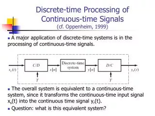
Post-processing of Continuous Shear Wave Signals

1. Post-processing of Continuous Shear Wave Signals April 28, 2011 EAS 4480 Taeseo Ku Civil & Environmental Engineering

2. Introduction 1. Shear wave velocity (Vs) • Second fastest wave & Directional and polarized • Most fundamental wave to geotechnical engineering • Depends on site-specific geostatic stress state 2. Applied data • ‘ConeTec, Inc.’ produced continuous shear wave measurements with depth to 45m at Richmond, BC (Seismic CPT) • Shear waves are collected at every 10cm vertical interval (Very short frequent interval !) • Sampling time = 0.05 msec fs = 20 kHz

3. Pump Horizontal Plank with normal load x t z1 Hammer z2 packer Horizontal Velocity Transducers (Geophone Receivers) R12 = z12 + x2 R22 = z22 + x2 Shear Wave Velocity: Vs = R/t Oscilloscope Downhole Testing Test Depth Interval Cased Borehole x

5. Post processing for continuous Vs signals • Signals are normalized by max. signal • Signal process : de-trend and filter the raw signals (low/high cutoff frequency pass) • A total of 418 data analyzed – bad signals are deleted • Butterworth filter - [b,a] = butter(n, Wn, 'type') • Input ▪ n: order of filter  n = 4 ▪ Wn: Cutoff frequency - use Nyquist frequency fNto normalize the input (fN= ½*fS= 10 kHz) ▪ Wn=[w1, w2]/fN, band filter [18Hz, 300Hz]/fN

7. Auto-covariance • • Auto-covariance for signal at 45.3 meter depth x = [x1, x2, …, xn] where xi is equally spaced in time

8. Power spectral density • • Power Spectral Density Estimate (signal at 45.3 meter depth) FFT fy = fft(y,nfft) f = 1/2*fs*linspace(0,1,n/2) Periodogram [Pxx,f] = periodogram(x,window,nfft,fs) LSSA : Lomb method [xp,xf] =lombscargle2(data,hifac,ofac) Observed Peak Frequency = 37.5 Hz

9. Post-processing for Vs – Time domain • • Example : cross-correlation method in time domain Time shift 0.0003 sec Time shift 45.2 & 45.3 meters Maximum covariance gives the time shift between two signals !

10. Post-processing for Vs – Frequency domain Cross spectral analysis [Pxy,F]=cpsd(x,y,window,noverlap,nfft,fs) Signals at 45.2 & 45.3 meter depth Observed peak frequency = 37.5 Hz Signals at 45.2 & 45.3 m depth Phase = angle(Pxy)/(2*pi)*360; interp1(F, phase, 37.5) Lag: 8.924 f = 37.5 Hz; T= 0.0267 sec ∆t = 8.924/360* 0.0267 = 0.000661 sec

11. Estimated Vs profile • • Sensitive • Time lags are very small • • Running-mean Filter for ∆t • Filter function: filtfilt • y = filtfilt (b, a, x) • describes filtering of vector x by • y(n) = b(1)*x(n) + b(2)*x(n-1) + ... + b(nb+1)*x(n-nb) • -a(2)*y(n-1) -... -a(na+1)*y(n-na) Generate a nth order running mean filter coefficient vector  b=1/(n+1)*ones(1,n+1);

12. Vs estimation using Running-mean filter 10th order running mean filter 15th order running mean filter

13. Relationship between Vs and depth of overburden • Empirical estimate from Lew & Campbell (1985, ASCE) • Relationships are derived for various Quaternary age soils • Over 270 Vs surveys including refraction, downhole , and crosshole • Regression analysis - Vs =K(d+c)n d : depth K,c, and n : constants dependent on geotechnical classification Average Vs Lew and Campbell,1985

14. Regression analysis (Time domain : n = 10) 10th order running mean filter Least-squares regression Vs = 120.86*(Depth)0.1882 (m/sec) Reduced major axis Vs = 74.51*(Depth)0.3539 (m/sec) Principal component Vs = 114.74*(Depth)0.2060 (m/sec) • Y = a∙Xc(Y = Vs, X = depth) • Transform to linear form • log(y) = c∙log(x) + log(a) • Correlation coefficient: r = 0.5317 • Coefficient of determination : R2 = r2 = 0.283

15. Regression analysis (Time domain : n = 15) 15th order running mean filter Least-squares regression Vs = 101.56*(Depth)0.2419 (m/sec) Reduced major axis Vs = 77.37*(Depth)0.3344 (m/sec) Principal component Vs = 97.82*(Depth)0.2547 (m/sec) • Y = a∙Xc(Y = Vs, X = depth) • Transform to linear form • log(y) = c∙log(x) + log(a) • Correlation coefficient: r = 0.7232 • Coefficient of determination : R2 = r2 = 0.523

16. Regression analysis (Frequency domain : n = 10) 10th order running mean filter Least-squares regression Vs = 64.75*(Depth)0.3834 (m/sec) Reduced major axis Vs = 58.94*(Depth)0.4156 (m/sec) Principal component Vs = 63.12*(Depth)0.3922 (m/sec) • Y = a∙Xc(Y = Vs, X = depth) • Transform to linear form • log(y) = c∙log(x) + log(a) • Correlation coefficient: r = 0.9225 • Coefficient of determination : R2 = r2 = 0.851

17. Regression analysis (Frequency domain : n = 15) 15th order running mean filter Least-squares regression Vs = 61.96*(Depth)0.3982 (m/sec) Reduced major axis Vs = 57.71*(Depth)0.4224 (m/sec) Principal component Vs = 60.71*(Depth)0.4051 (m/sec) • Y = a∙Xc(Y = Vs, X = depth) • Transform to linear form • log(y) = c∙log(x) + log(a) • Correlation coefficient: r = 0.9427 • Coefficient of determination : R2 = r2 = 0.889

18. Summary • Post processing for continuous Vs signals ▪Detrend data & band pass filtering ▪ Auto-covariance, PSD estimate • Vs evaluated by ‘cross-correlation’ & ‘cross-spectral analysis’ ▪ Time domain : find max. covariance between signals ▪ Frequency domain : cross spectral analysis – phase lags ▪ Sensitive results : apply nth order running-mean filter • Regression analysis ▪ Transform to linear form (Vsvs depth) ▪ LS regression, RMA regression , PC regression