Download
1 / 26
260 likes | 362 Vues
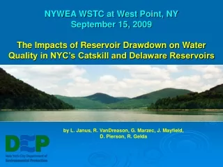
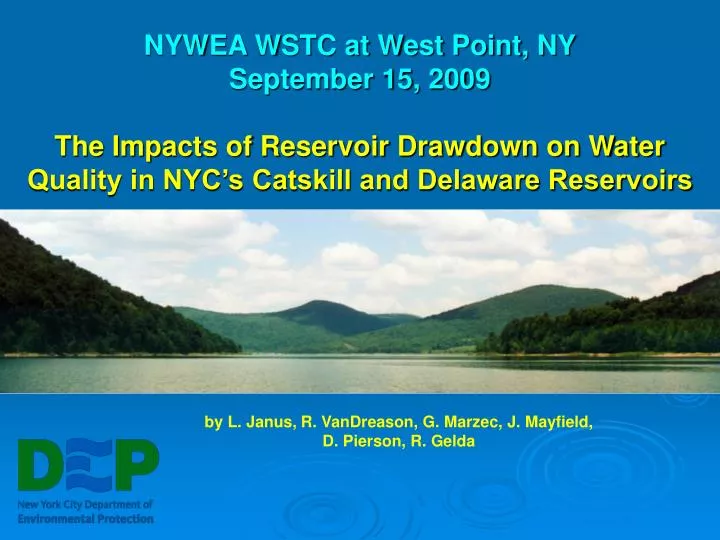
NYWEA WSTC at West Point, NY September 15, 2009 The Impacts of Reservoir Drawdown on Water Quality in NYC’s Catskill and Delaware Reservoirs. by L. Janus, R. VanDreason, G. Marzec, J. Mayfield, D. Pierson, R. Gelda. Impacts of Drawdown on Water Quality. Outline: 1.0 Introduction

E N D
NYWEA WSTC at West Point, NY September 15, 2009 The Impacts of Reservoir Drawdown on Water Quality in NYC’s Catskill and Delaware Reservoirs by L. Janus,R. VanDreason, G. Marzec, J. Mayfield, D. Pierson, R. Gelda
Impacts of Drawdown on Water Quality Outline: 1.0 Introduction • Why is drawdown important? • How was the analysis conducted? 2.0 Hydrology and water quality • Elevation histories • Water residence times – headwaters vs terminal • Relation of hydrodynamics to WQ 3.0 Reservoir WQ observations: • Time series plots: 20-years of water quality • WQ vs elevation relationships • ‘Breakpoints’ and correlations 4.0 Diagnostic Modeling • Ashokan – 2008 drawdown • West Branch during 2008 drawdown 5.0 Conclusions
1. Introduction Objectives: • Define how and when DEP reservoirs respond to drawdown. • Determine elevation ‘targets’ that are protective of WQ. • Understand how drawdown or prolonged drought might affect WQ. • Gain insight into impacts of climate change. Approach: • literature review - nation-wide • Review hydrodynamics • Relate elevations to reservoir WQ • Time series behavior • Correlations of WQ with elevations • Analyze case studies of specific events • diagnostic modeling
Literature Review • Nationwide review; studies have demonstrated: • Increased sediment resuspension occurs at a threshold level. • Impacts on algal dynamics with increases in chlorophyll • Impacts on the thermal structure, with decreases in the duration of stratification. • changes to benthic invertebrate communities • impacts on fish populations • 3 NYC Watershed Studies: • Effler & Matthews, 2004; Effler & Bader, 1998; Effler, et al., 1998 • Major drawdown at Cannonsville in 1995 demonstrated: • Increased tripton (suspended particles other than algae) • Increased turbidity • Increased phosphorus • Enhanced phytoplankton growth • Decreased Secchi depth
2.0 Hydrology and water quality Configuration of NYC’s Catskill and Delaware Reservoirs: Map by D. Lounsbury - terminal reservoirs receive flow from upstream headwater reservoirs
Catskill Reservoirs - elevation and storage histories: Schoharie West Basin Ashokan Water Surface Elevation (meters above sea level) Proportion of Available Storage East Basin Ashokan
Cannonsville Pepacton Water Surface Elevation (meters above sea level) Proportion of Available Storage Neversink Rondout
Water Residence Times - 30 years (Volume/Hydraulic load = replacement rate)
How does hydrology affect water quality? History: • equations developed in 1960s by Vollenweider • basis of OECD solution to eutrophication problems in Europe • basis of TMDLs in the US • Late 1960s National Eutrophication Survey by USEPA • 1981 EPA issued Restoration of Lakes and Inland Waters resulting from conference in Portland, Maine • 1983 Chapra & Reckhow explored refinements – sedimentation Hydrology is a determinant of Water Quality: • Hydraulic loads determine water residence times, nutrient loads, and reservoir nutrient concentrations • Water residence times are a primary determinant of nutrient concentrations and influence primary production, turbidity, and Secchi depths
Critical phosphorus load - is a function of depth and hydraulic load. - shallower lakes tolerate lower nutrient loads (from Vollenweider, 1976)
Observations on hydrology of NYC reservoirs: • Reservoirs typically have shorter water residence times than lakes (average of 1.3 years for North American lakes). • Terminal reservoirs show very stable elevations and water residence times (with the exception of drought periods). • Terminal reservoirs have greater hydraulic loads than upstream reservoirs, and therefore shorter water residence times. More rapid flushing benefits WQ. • Headwater (upstream) reservoirs are more frequently drawn down than terminal (downstream) reservoirs, therefore provide insight into WQ changes due to drought.
3.0 Water Quality: potential impacts of drawdown cited in the literature were explored with reservoir data: • Turbidity • Conductivity • Eutrophication indicators: (Secchi depth, nutrients, algae) • Bacteria – fecal coliforms
Scatter Plot Analysis Methodology: • Monthly (April-December) reservoir medians using all sample depths and sites from1988-2007 • Only elevations 0.5 ft below spill considered • LOWESS curves shown • Spearman correlations • Non-parametric ranking • P<0.05 R= -0.71
Cannonsville Scatter Plots R= -0.71 R= 0.50 R= -0.11 (ns) R= -0.30 R= -0.55 R= -0.66
Pepacton Scatter Plots R= -0.46 R= 0.33 R= -0.10 (ns) R= 0.59 R= -0.47 R= -0.33 R= -0.32 R= -0.20 R= -0.51
Neversink Scatter Plots R= -0.36 R= 0.51 R= -0.37 R= -0.68 R= 0.63 R= -0.44 R= -0.12 R= -0.47 R= -0.37 R= -0.28
Water quality variables vs. elevation correlations with r > 0.50 (r values shown were highest at the designated elevation range) Note: There were no examples where chlorophyll a had an r of > 0.5
Waterfowl in the East Basin of Ashokan – coincident with high fecal coliform bacteria
4.0 Two Examples of diagnostic modeling: Example 1. Ashokan Example 2. West Branch • Both occurred during a Rondout–West Branch Tunnel valve repair in 2008. • Both analyses depended on high frequency monitoring.
Example 1. Ashokan: Simulated Turbidity Compared to Turbidity Measured in the Reservoir by Robotic Monitoring • Model simulations that include resuspension more closely match measured data. • Wind driven shoreline resuspension is important.
What does wind resuspension look like?This photo shows resuspended clays in Schoharie Reservoir. Note photos on right:very sensitive even when nearly flat calm
Example 2. West Branch - High Frequency Monitoring of Turbidity (black) and elevation (red) during 2008 Delaware Aqueduct Shutdown Mean Daily Turbidity vs. Water Surface Elevation • Conclusion: • These data clearly link drawdown to increased turbidity • Turbidity nearly doubles, but levels only reach 4 NTU
5. Conclusions • Water quality is affected negatively by reservoir drawdown. • Draw-down affects flushing rates, which in turn affect water quality. • Headwater reservoirs are more frequently drawn down than terminal reservoirs due to operations; this benefits WQ as it approaches intakes. • Time series and correlations of WQ data showed correspondence to elevation, but with high variability. • Secchi depth and turbidity showed the highest correlations to elevation. • Diagnostic modeling provided insight into the role of wind-driven resuspension. • Models are essential in deciphering functional relationships between dynamically changing parameters.
Thank Youwww.nyc.dep.gov Acknowledgements: D. Kent, and Y. Tokuz for literature search, D. Lounsbury for map, C. Nadareski and M. Reid for waterfowl info, WQD field and lab staff for historic data, and UFI for modeling work