Download
1 / 35
350 likes | 494 Vues
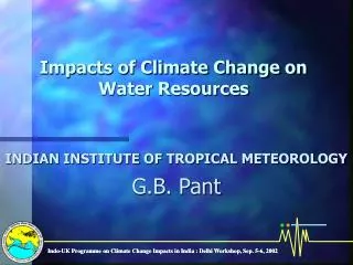
5 th International Symposium on Integrated Water Management Nanjing, China, November 19-21, 2010. A Physically-based Approach to Assess the Impact of Climate Change on Canadian Water Resources. Edward A. Sudicky, Jianming Chen and Young-Jin Park

E N D
5th International Symposium on Integrated Water Management Nanjing, China, November 19-21, 2010 A Physically-based Approach to Assess the Impact of Climate Change on Canadian Water Resources Edward A. Sudicky, Jianming Chen and Young-Jin Park Department of Earth and Environmental Sciences, University of Waterloo, Waterloo, ON, Canada W. Richard Peltier Department of Physics, University of Toronto, Toronto, ON, Canada
Climate Change and Water Resources in Canada • Evidence of climate change is mounting. • Water demand will continue to increase while water quality keeps deteriorating. • Two critical questions rise: • What are the plausible impacts that future climate change may have on our water resources? • What adaptive strategies can be implemented to mitigate such impacts? • A science-based framework that fully-integrates climate change & surface/subsurface flow is relevant to sound policy decisions, particularly at continental & trans-border scales.
An Inconvenient Truth... or Convenient Fiction? Climate Change The entire global scientific community has a consensus on the question that human beings are responsible for global warming and he [Bush] has today again expressed personal doubt that that is true. Doubt it
Water Cycle and Global Water Distribution Atmospheric Water (0.04%) Frozen water (69%) Surface Water (0.3%) Fresh water Saline Water (98%) Ground Water (30%)
Integrated Physically-Based Modelling Attempt to account for all interactions between surface and subsurface flow regimes Conceuptually Superior to linked simulators or iteratively coupled simulators Complex (more processes, highly nonlinear)
Challenges • Disparate time frames between atmospheric/surface/subsurface flow and transport regimes, myriad of processes • Very large unstructured grids, irregular topography, complex boundary conditions, surface properties & geological features • Strong nonlinearities in governing equations • Data availability and upscaling issues
Some Issues • How well can we represent all the relevant processes in a scientifically plausible, physically-based manner? • How big can we go in 3D, and over what time frames? • Do we have the needed input data and, if not, how do we acquire it? • What linkages should be made to other disciplines (atmospheric science, agriculture, geomorphology, biology, ecology, economics, policy & decision making…)? • What are the key scientific & societal questions to be addresses?
Examples of Coupled Surface-Subsurface Models Earliest known coupled surface/subsurface flow model: Freeze, R.A. and R.L. Harlon, Blueprint for a physically-based, digitally-simulated hydrologic response model, J. Hydrol., 9, 237-258, 1969. Some Existing “Integrated” Models: • InHm • MODHMS • HydroGeoSphere • Parflow • OpenGeoSys • … Seems to be a growing area of model development, but do we need more models, or more applications centered on resolving key societal concerns & scientific questions
Overview of Current “HydroGeoSphere” Model Features • 2D overland/stream flow (Diffusion-wave equation), including stream/surface drainage network genesis; • 3D variably-saturated flow (Richards’ equation + ET) in porous medium; • 3D variably-saturated flow in macropores, fractures and karst conduits (dual-porosity, dual-permeability or discrete fractures); • Advective-dispersive, reactive solute/thermal transport in all continua, snow accumulation/melting, soil freeze/thaw; • Groundwater age, life expectancy (Park et al., WRR, 2008; Cornaton et al., WRR, 2008); • Allows for complex topography, irregular surface & subsurface properties, density-dependent flow, subgridding & subtiming (Park et al., AWR, 2008; Park et al., VZJ,2009), parallel version; • Fully-coupled, simultaneous solution of surface/subsurface flow and transport via Control-Volume Finite Element or Finite Difference Methods.
Selection Climate Models • Community Climate System Model (CCSM), which is primarily supported by the US National Centre for Atmospheric Research (NCAR) • Downscaling of CCSM3.0 is currently performed at the SciNet, a new HPC facility based at the University of Toronto, fastest in Canada and within top 10 in the world • Canadian Regional Climate Model (CRCM), which provides downscaled data at ~45 km resolution, will be selected for comparison
Community Climate System Model (CCSM) Atmosphere Coupler Land HydroGeoSphere Ice Ocean
Influence of Climate Change on Water Resources in Regional-Scale Watersheds: An example in the Grand River Watershed
Calibration for Long-Term Averages Stream Discharge Subsurface Head Observed Simulated Surface Drainage Networks
Depth to Water Table [m]: Driest vs. Wettest Scenarios Scenario 1: Driest Scenario 5: Wettest
ET precipitation geology soil type sediment thickness land use 3D Simulations over the Canadian Landmass
3D Hydrogeology & FE Mesh Continuous permafrost Discontinuous permafrost Upper unconsolidated sediment Lower unconsolidated sediment Sedimentary rock Fractured basement rocks Basement rocks
Calibration for the Averages of 1961-2000 Major Lakes Water Level Major Rivers Stream Discharge Simulated Surface Water Depth Distribution Map of Observed Major Rivers and 10 Largest Lakes
HGS Infiltration/Exfiltration Compared to CCSM3.0 (Present-Day) Exchange Flux by HGS Infiltration Flux by CCSM3.0 - Infiltration + Discharge
CRCM4.2 (~45 km) CCSM3.0 (~155 km) Projection in 2099 Stream Discharge Decrease Increase Change in Water Depth CRCM4.2 (~45 km) CCSM3.0 (~155 km) Change in Net Precipitation Decline Rise Change in Water Table Elevation
Summary Potential impacts of climate change on Canadian water resources: • a decline in water levels in both inland lakes and four Great Lakes, • less groundwater recharge, dry-up of small streams, reduced wetland area, poorer water quality, and less wildlife habitat due to reduced summer water levels • an increase in the frequency and severity of droughts and flooding. • in the areas of Canadian Prairie, declined streamflow and more frequent droughts will have a significant impact on the efficiency of farming, heavily relying on irrigation. • Permafrost melting is one of the most striking and visual signs of the impacts of climate change in Canada.
Gridding Issues in Fully-Integrated Hydrologic Simulation at the Watershed->Continental Scale
Motivation • It is inevitable to use relatively large grid sizes when simulating at these large scales given the current level of computing hardware performance. • Two legitimate questions rise: • What does the coarse-grid simulation result really represent? i.e. same as the average of fine-grid simulation? • How to maximize the similarity between the coarse-grid result and the fine-grid result?
Summary of Simulations • Test cases based on Grand River Basin • Five different sizes of plan-view grids (200m, 1km, 2km, 5km and 10km), but with • For comparison purpose, both nearest-neighbour DEM and hydrologically bi-linear (FE) least squares fit (hydrologically-best-fit) elevationsare used in 1, 2, 5 and 10 km grid simulations. • Finite difference method, fully-integrated, variably-saturated subsurface flow.
Hydrologically Bi-linear (FE) Least Squares Fit Topography vs. Actual Topography • In general, weighting of each DEM point is inversely proportional to its distance to the node • Hydrologically important features, i.e. major streams, receive much higher weighting in calculation DEM resolution: 200 m Grid size: 10 km
Nearest vs. Hydrologically-Best-fitDepth to Water Table (m) 1km 2km Nearest 200m 1km 2km (Assumed as the reality) Best-fit
Nearest vs. Hydrologically-Best-fitDepth to Water Table (m) 5km 10km Nearest 200m 5km 10km (Assumed as the reality) Best-fit
New Depth to Water Table Derived from 200m DEM and Water Table Elevation from Coarse Grid Simulation Original result of 200m grid simulation Derived from DEM and WT elevation of 5km grid simulation Original result of 5km grid simulation (Assumed as the reality) Depth to Water Table (m) Derived from DEM and WT elevation of 10km grid simulation Original result of 10km grid simulation
Nearest vs. Hydrologically-Best-fitExchange Flux (mm/year) 1km 2km Nearest 200m Exfiltration 1km 2km Infiltration (Assumed as the reality) Best-fit
Nearest vs. Hydrologically-Best-fitGroundwater Recharge/Discharge (mm/year) 1km 2km Nearest Discharge 200m 1km 2km Recharge (Assumed as the reality) Best-fit
Summary of Groundwater Recharge Results • Hydrologically-best-fit topography is used • Rate of net precipitation: 400 mm/year • Area of entire simulation domain: 4300 km2
Method for calculation of new surficial soil moisture • New depth to water table at the original DEM resolution is computed by the following equation: New_Depth2WT = Max{(Fine DEM – Course Grid WT elevation), 0.0} • Depth2WT vs. Saturation table is computed based on the result of an 1D unsat simulation with the same parameters and infiltration as the 3D simulation. • Surficial soil moisture content data is then determined by the new depth to water table and the Depth2WT-Saturation table.
New Surficial Soil Moisture Content Data Original result of 200m grid simulation Derived from new Depth2WT of 1km grid simulation Derived from new Depth2WT of 2km grid simulation (Assumed as the reality) Surficial Saturation Derived from new Depth2WT of 5km grid simulation Derived from new Depth2WT of 10km grid simulation