Download

1 / 69
700 likes | 839 Vues
Water, salt, and heat budget. ●Conservation laws application: box models ●Surface fresh water flux: evaporation, precipitation, and river runoff ●Surface heat flux components: sensible, latent, long and shortwave ●Ocean meridional transport. Mass Conservation. Continuity equation.

E N D
Water, salt, and heat budget ●Conservation laws application: box models ●Surface fresh water flux: evaporation, precipitation, and river runoff ●Surface heat flux components: sensible, latent, long and shortwave ●Ocean meridional transport
Mass Conservation Continuity equation
Mass Conservation Continuity equation , total mass in a column, we have Integrating in ocean depth, , where . Vertical boundary conditions: E-evaporation, P-precipitation, R-river runoff (measured in m/s, 1mm/day=1.1574x10-8 m/s). Melting of sea ice may also be a factor (neglected here)
Gaussian formula: Integrating a two dimensional vector field over an area S with boundary L, we have Where is a unit vector perpendicular to the boundary L. Define the mass in a water column of bottom area as S: Integrating the continuity equation in S with boundary L: Using Gaussian formula
Lateral boundary conditions: If L is a closed basin (e.g., the coastal line of an ocean domain): no slip condition: on L. free slip condition: In both cases Then
Salt Conservation , vertical eddy diffusion coefficient. , horizontal eddy diffusion coefficient. The molecular diffusivity of salt is Ratio between eddy and molecular diffusivity: Integrating for the whole ocean column,
We have known that and However, both E and P transfer the fresh water with S=0 There is a net salt influx into the oceans from river runoff (R), which is totally about 3 x 10¹² kg/year. About 10% of that is recycled sea salt (salt spray deposited on land). The turbulent salt flux through the surface and at the bottom of the sea are small (entrainment of salt crystals into atmosphere) (subsidence at the bottom, underwater volcano-hydrothermal vents) Compared to the total salt amount in the ocean: 5 x 10¹⁹ kg, the rate of annual salt increase is only one part in 17 million/year. As we know, the accuracy of present salinometer is ±0.003. Given average salinity 35 psu, the instrument uncertainty is in the order of ±0.003/35=1500/17 million. The amount is small and negligible for salt budget. Overall,
There is a net vertical salt flux near the sea surface driven by the fresh water flux. Consider a thin interfacial layer, the balance of fresh water flow is Where m is the rate of volume of the sea water entrained into the thin layer from its bottom The corresponding turbulent salt flux is or Where So is usually chosen as 36‰. Usually, we neglect the effect of E-P on mass balance (i.e., w(z=0)=0) and take into its effect on salinity as Apparent salt flux
Box Model Under steady-state conditions, we apply the conservations of mass and salt to a box of volume V filled with sea water. Conservation of volume: Where Vi is inflow, Vo outflow; P precipitation, E evaporation, and R river runoff. Salt conservation: influx outflux
Denote excess fresh water as Since With , we have and If Si≈So, (Vi , Vo) » X. Large exchange with the outside. If Si » So, Vi « X. Vo slightly larger than X. Small exchange.
An evaporation rate of 1.2 m/yr is equivalent to removing about 0.03% of the total ocean volume each year. An equivalent amount returns to the ocean each year, about 10% by way of rivers and the remainder by rainfall. The yearly salt exchange is less than 10-7 of the total salt content of the ocean.
Heat budget Temperature (Potential Temperature) Equation . where : specific heat capacity at constant pressure. , vertical eddy diffusion coefficient. , horizontal eddy diffusion coefficient. , Molecular thermal diffusivity . ( ) Define , we have and
, heat storage. , heat convergence by currents and sub-scale transport. , penetrating solar radiation. , surface heat flux. Qsa: solar radiation absorbed at the sea surface. Qb: net heat loss due to long wave radiation. Qe: latent heat flux. Qh: sensible heat flux. , geothermal heat flux (neglected). We also take Qs=Qsp+Qsa as total solar radiation. Then the heat budget is:
Solar radiation: Basics Planck’s law: Black body irradiance (absorptance ) h~ Planck’s constant. k~ Boltzmann’s constant. c~ light speed in vacuum. T~ temperature (Kelvin), λ~wavelength. Total irradiance (Stefan-Boltzmann law): Stefan-Boltzmann constant: The wavelength of maximum irradiance (Wien’s law): Temperature at sun’s surface: T=5800K λm=0.5μm. , Solar radiation is in shortwave band: 50% visible, 0.35μm ≤ λ ≤ 0.7μm; 99%, λ ≤ 4μm
Solar flux at the top of the atmosphere: FS=1365-1372 W/m2 Solar constant: (mean solar flux on 1 square meter of earth) Usually, we choose . Not all of the radiation received at the top of atmosphere is available to the ocean
If the incoming radiation is normalized to 100%, then 16% are absorbed in the atmosphere 24% are reflected by clouds 7% are radiated back to space from the atmosphere 4% are reflected from the earth's surface (mainly from the sea) The rest into the ocean (49%)
Factors influencing QS 1). Length of the day (depending on season, latitude) 2). Atmospheric absorption. Absorption coefficient (gas molecules, dust, water vapor, etc). Elevation of the sun θ: angle of the sun above the horizon. 3). Cloud absorption and scattering. 4). Reflection at the sea surface. direct sunlight (from one direction) reflection depends on elevation of the sun and the state of the sea (calm or waves). skylight (scattered sunlight from all directions) reflected about 8%. (A few percent of the radiation entering the sea may also be scattered back to the atmosphere)
Empirical Formula (Parameterization) (shortwave flux averaged over 24 hours): Qso is clear sky solar radiation at sea surface. F is an empirical function of the fractional cloud cover. Example: 1). Clear sky radiation QSO: clear sky radiation. An: noon altitude of the sun in degree. tn: length of the day from sunrise to sunset in hours. 2). Cloud reduction is the solar flux arriving at the sea surface. C=8, C=4, 3). Reflection at the sea surface 4). Shortwave radiation into the sea 5). Original algorithm overestimates. Multiply by 0.7.
Another example: Reed (1977) n~ fractional cloud cover (0.3 ≤n≤1). Otherwise Qs=Qso. φ~ solar elevation in degrees. cn~ cloud attenuation factor (≈0.62). α~ albedo.
Distribution daily inflow of solar radiation • The highest value (>300 W/m2) occur at 30oS and 30oN in respective summer hemispheres. • There is no shortwave input at high latitudes during the polar winter. • The amount of energy input is greater in the southern hemisphere than in the northern hemisphere. (In its elliptic orbit, earth is closer to the sun in southern summer).
Absorption in the sea reduces the light level rapidly with depth. 73% reaches1 cm depth 44.5% reaches1 m depth 22.2% reaches10 m depth 0.53% reaches100 m depth 0.0062% reaches200 m depth
Long-wave radiation (Qb) The difference between the energy radiated from the sea surface (σT4, T ocean skin temperature) and that received from the sea by the atmosphere, mostly determined by water vapor in lower atmosphere. The outgoing radiation from the sea is always greater than the inward radiation from the atmosphere. Qb is a heat loss to ocean. The outgoing radiation is “longwave” Mean sea surface temperature is T= 12oC=285K, λm=10.2μm. Most of the longwave radiation is in the range 3μm ≤ λ ≤ 80μm Longwave radiation is much smaller than the shortwave solar radiation
Empirical Formula of Qb tw=water temperature (oC). ea=relative humidity above the sea surface. C=cloud cover in oktas (1-8). Qbo=Qb(C=0) ranges from 70-120 W/m2. Qb (Qbo) decreases with tw and ea. ea increases exponentially with tw. Due to the faster increase of ea, inward atmospheric flux is larger than outgoing surface radiation). The net heat loss decreases with tw.
Another formula: ε=0.98, λ increases with latitude (0.5, equator; 0.73, 50o). e water vapor pressure (mb): Saturated water vapor pressure Nonlinearity in water vapor dependence: The water vapor content (humidity) increases exponentially with TS, which could result in a more rapid increase in the atmosphere’s radiation into the sea than the sea’s outward radiation (proportional to TS4. Thus Qb could decrease as TS increases, leading to a “super greenhouse” effect. It should be noted that this is still a highly speculated process, which has not been substantiated with a significant amount of measurements.
Properties of long wave radiation • Qb does not change much daily, seasonally, or with location. This is because (1) Qb ~T4, for T=283K, ΔT=10K, , which is only 15% increase. (2) Inward radiation follows outgoing radiation. • Effect of cloud is significant. The big difference between clear and cloudy skies is because the atmosphere is transparent to radiation range from 8-13μm while clouds are not. • Ice-albedo feedback Effect of ice and snow cover is relatively small for Qb but large for Qs due to large albedo (increase from normally 10-15% to 50-80%). Therefore, net gain (Qs-Qb) is reduced over ice. ice once formed tends to maintain.
Evaporative heat flux (Qe) 51% of the heat input into the ocean is used for evaporation. Evaporation starts when the air over the ocean is unsaturated with moisture. Warm air can retain much more moisture than cold air. The rate of heat loss: Fe is the rate of evaporation of water in kg/(m2 s). Lt is latent heat of evaporation in kJ. For pure water, . t~ water temperature (oC). t=10oC, Lt=2472 kJ/kg. t=100oC, Lt=2274 kJ/kg. In general, Fe is parameterized with bulk formulae: Ke is diffusion coefficient for water vapor due to turbulent eddy transfer in the atmosphere. It is dependent on wind speed, size of ripples, and waves at sea surface, etc. de/dz is the gradient of water vapor concentration in the air above the sea surface.
In practice: V wind speed (m/s) at 10 m height above sea. es is the saturated vapor pressure over the sea-water (unit: kilopascals) The saturated vapor pressure over the sea water (es) is smaller than that over distilled water (ed). For S=35, es=0.98ed(ts). ea is the actual vapor pressure in the air at a height of 10 m above sea level. If the atmospheric variable is relative humidity (RH), ea=RH x ed(ta). Example: Ta=15oC, ed = 1.71 kPa = 12.8 mm Hg, RH=85%, then ea= 1.71 x 0.85 kPa= 1.45 kPa. This empirical formula is an approximation of eddy diffusion formula because: , and (very crude parameterization).
In most region, es > ea, Fe and Qe are positive, there is a heat loss from the sea due to evaporation. • In general, if ts-ta > 0.3oC, Qe >0. • In some region, ts-ta<0oC (surface air is warmer than SST) and RH is high enough to cause condensation of water vapor from the air into the sea, which results in a gain of heat in the sea. Fogs occur in these regions due to the cooling of the atmosphere over the sea.
Sensible heat flux (Qh): On average, the ocean surface is about 0.3-0.8°C warmer than the air above it (exception: upwelling regions). Direct heat transfer (transfer of sensible heat) therefore occurs usually from water to air and constitutes a heat loss. Heat transfer in that direction is achieved much more easily than in the opposite direction for two reasons: 1. It takes much less energy to heat air than water. The energy needed to increase the temperature of a layer of water 1 cm thick by 1°C is sufficient to raise the temperature of a layer of air 31 m thick by the same amount. 2. Heat input into the atmosphere from below causes instability (through a reduction of density at the ground) which results in atmospheric convection and turbulent upward transport of heat. In contrast, heat input into the ocean from above increases stability (through a reduction of density at the surface) and prevents efficient heat penetration into the deep layers.
Empirical formula of Qh Bulk formula: Wyrtki (1965): ρa = 1.2 kg/m3 (density of air). Cd = 1.55 x 10⁻³ (drag coefficient at sea surface). V surface (10 m) wind speed in m/s. Cp=1008 J/(kg K). Then .
More recent bulk formula (Smith 1988): Surface latent heat flux where is specific humidity Surface sensible heat flux . Ke and Kh are mainly functions of stability and wind speed. Ke≈1.20Kh