
2.2 Hyperbolic PDEs
E N D
Presentation Transcript
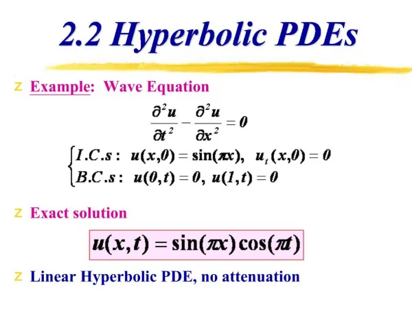
1. 2.2 Hyperbolic PDEs Example: Wave Equation
Exact solution
Linear Hyperbolic PDE, no attenuation
3. 2.2.1 Interpretation by Characteristics Consider the Wave equation
Two real roots (two characteristics)
Two characteristic lines
4. Method of Characteristics Develop computational grid and numerical solutions along the characteristic directions (? = x ? ct, ? = x + ct)
General solutions - preserve the functional forms (f and g) along the characteristic lines during propagation
In (x,t) coordinates, ? is a function of space and time, propagation with finite speed u = dx /dt = ? c
In (?,?) coordinates, the wave appears to be stationary
No attenuation (diffusion/dissipation) or dispersion (distortion of wave shape)
Discontinuity will propagate into the flow domain
5. 2.2.2 Interpretation on a Physics Basis Hyperbolic equation � propagation problem with no dissipation
6. Hyperbolic PDEs Wave equation
Canonical form
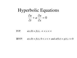
Consider a pure initial value problem with ?(x,0) = S(x), ?t (x,0) = cT(x)
7. Hyperbolic PDEs Initial wave forms
Exact solution
8. Method of characteristics
The solution at P(xi,tn) is uniquely determined by the initial conditions S(x) and T(x) Hyperbolic PDEs
9. 2.2.3 Appropriate Boundary (and Initial) Conditions General rule for hyperbolic PDEs
The number of auxiliary conditions is equal to the number of characteristics pointing into the domain
Case (A): Both auxiliary conditions given on a non-characteristic curve
Case (B): One auxiliary condition on a characteristic curve
Case (c): Both auxiliary conditions on characteristic curves
10. Auxiliary conditions Case (A): Both auxiliary conditions on a non-characteristic curve
11. Auxiliary conditions Case (B): One auxiliary conditions on a characteristic curve
12. Auxiliary conditions Case (C): Both auxiliary conditions on characteristic curves
13. Characteristics - Propagation Domain of Dependence
14. Characteristics - Propagation Domain of Influence
15. 2.3 Parabolic PDEs Both the hyperbolic and parabolic PDEs are associated with propagation problems
Hyperbolic � propagation problems without attenuation
Parabolic � include dissipative (diffusive) mechanisms
16. 2.3.1 Interpretation by Characteristics Consider ut + uux = ? uxx
B2 � 4AC = 0 : Parabolic
One characteristic direction defined by dt/dx = 0
The characteristic dt/dx = 0 never advance the solution in time, no equivalence to the method of characteristics for parabolic equations
Hyperbolic � advance the solutions in (?,?) directions
17. Parabolic PDEs Parabolic � never advance the solution in time, disturbance propagates immediately (with infinite speed) to every part of the solution domain at any given time t
18. 2.3.2 Interpretation on a Physical Basis Typical parabolic problems �march forward in time, but diffusive in space
Dissipative � disturbance attenuates quickly away from point P
e?kx decay exponentially, but non-zero in the entire domain
19. 2.4 Elliptic PDEs Examples
A=1, B=0, C=1, B2 � 4AC = � 4 < 0
Elliptic � no real characteristics
Maximum principle: both the maximum and minimum values of ? must occur on boundary
Mean Value Theorem:
20. 2.4.1 Interpretation by Characteristics The characteristics cannot be displayed in the (real) computational domain
Identification of characteristics serves no purpose (no propagation behavior)
Every direction is equally important
Equilibrium problems
When ? is small, the first order terms exhibit propagation behavior along dy/dx = v/u
21. 2.4.2 Interpretation on a Physics Basis Equilibrium (Jury) problems
A disturbance introduced at P influences all other points in the domain
The influence usually diminishes away from P
It is necessary to consider global solution domain (rather than marching)
Discontinuity in auxiliary data are smoothed out in the interior (smooth solution)
Boundary conditions are required on all boundaries (may be any combinations of Dirichlet, Neumann or mixed conditions)
However, if Neumann conditions are used on all boundaries, then the Green�s theorem must be satisfied
22. Elliptic PDEs Domain of Dependence coincides with the domain of influence