Download
1 / 90
950 likes | 1.28k Vues
Measurement and Interpretation of Elasticities. Chapter 5. Discussion Topics. Own price elasticity of demand Income elasticity of demand Cross price elasticity of demand Other general properties Applicability of demand elasticities. Key Concepts Covered….

E N D
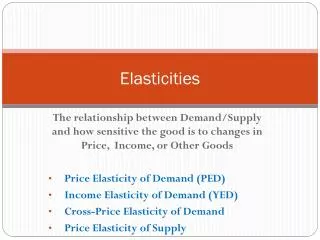
Discussion Topics • Own price elasticity of demand • Income elasticity of demand • Cross price elasticity of demand • Other general properties • Applicability of demand elasticities
Key Concepts Covered… • Own price elasticity = %Qbeeffor a given%Pbeef • Incomeelasticity = %Qbeeffor a given%Income • Cross priceelasticity = %Qbeeffor a given%Pchicken Pages 91-95
Key Concepts Covered… • Own price elasticity = %Qbeeffor a given%Pbeef • Incomeelasticity = %Qbeeffor a given%Income • Cross priceelasticity = %Qbeeffor a given%Pchicken • Arc elasticity = range along the demand curve • Point elasticity = point on the demand curve Pages 91-95
Key Concepts Covered… • Own price elasticity = %Qbeeffor a given%Pbeef • Incomeelasticity = %Qbeeffor a given%Income • Cross priceelasticity = %Qbeeffor a given%Pchicken • Arc elasticity = range along the demand curve • Point elasticity = point on the demand curve • Price flexibility = reciprocal of own price elasticity Pages 91-95
Own Price Elasticity of Demand We have the choice of focusing on the elasticity at a specific point on the demand curve or the elasticity over a relevant range on the demand curve Arc elasticity Point elasticity Single point on curve Relevant range on curve Pb Pa Pa Qb Qa Qa Page 91
Own Price Elasticity of Demand Our focus in this course will be on Arc Elasticity, or the response in quantity demanded as a result of a given change in the price of the product over a relevant range of the demand curve. Arc elasticity Relevant range on curve Pb Pa Qb Qa Page 91
Three approaches… Own price elasticity of demand Percentage change in quantity Equation 5.1 = Percentage change in price Own price elasticity of demand (QA – QB) ([QA + QB] 2) (PA – PB) ([PA + PB] 2) Equation 5.2 = Own price elasticity of demand = [QP] × [PQ] Equation 5.3 Page 91
Three approaches… Own price elasticity of demand Percentage change in quantity Equation 5.1 = Percentage change in price Own price elasticity of demand Given enough information, all three approaches give the same answer [QA – QB ([QA + QB] 2) [PA – PB ([PA + PB] 2) Equation 5.2 = Own price elasticity of demand = [QP] × [PQ] Equation 5.3 Page 91
First approach… Own price elasticity of demand Percentage change in quantity Equation 5.1 = Percentage change in price If you know the percentage change in quantity over a range on the demand curve associated with a given percentage change in price, you can calculate the elasticity. For example, if movie ticket sales drop by 40 percent as a result of a 22 percent increase in ticket prices, the elasticity would be -1.8, or -1.8 = -.40 ÷ .22 Interpretation: A 1% increase (decrease) in price would cause quantity demanded to drop (rise) by 1.8 percent. Page 91
First approach… Own price elasticity of demand Percentage change in quantity Equation 5.1 = Percentage change in price Alternatively, if you know the elasticity associated with ticket sales is -1.80 and have been informed that the theater is planning to raise prices 22 percent, you can solve for the percentage change in the quantity of ticket sales, or: -1.80 = %Q ÷ .22 %Q = -1.80 × .22 = - .40 or - 40% Thus ticket sales will drop by 40% if the theater raises ticket prices by 22%. Page 91
Second approach… Own price elasticity of demand [(QA – QB) ([QA + QB] 2) [(PA – PB) ([PA + PB] 2) Equation 5.2 = The subscript “a” here stands for “after” while “b” stands for “before”. The numerator represents the percent change in quantity over the range of the demand curve associated with Qa and Qb. The denominator represents the percent change in price over the same range. Pb Pa Qb Qa Page 91
Second approach… Own price elasticity of demand [(QA – QB) ([QA + QB] 2) [(PA – PB) ([PA + PB] 2) = Equation 5.2 Suppose the quantity demanded fell from 3 to 2 when the price increased from $1.00 to $1.25, or: PB = $1.00 QB = 3 PA = $1.25 QA = 2 Substituting these values into the equation above, we see the elasticity over this range would be: -1.8 = (2 – 3) 2.5 ($1.25 – $1.00) $1.125 Page 91
Second approach… Own price elasticity of demand [(QA – QB) ([QA + QB] 2) [(PA – PB) ([PA + PB] 2) = Equation 5.2 (2 – 3) 2.5 ($1.25 – $1.00) $1.125 = - 1.8 Thus if the quantity demanded fell from 3 to 2 when the price increased from $1.00 to $1.25, the elasticity over this range would be -1.8. This suggests that a one percent increase in pricewould reduce the quantity demanded by 1.8 percent!!! Page 91
Second approach… Own price elasticity of demand [QA – QB ([QA + QB] 2) [PA – PB ([PA + PB] 2) = Equation 5.2 [2 – 3 ([3 + 2] 2) [$1.25 – $1.00 $1.125]) = - 1.8 Alternatively, if you were given the elasticity and told that the price increased from $1.00 to $1.25, you can calculate the percentage change in quantity demanded by: - 1.8 = %∆Q ÷ [($1.25 – $1.00) $1.125] %∆Q = (-1.8) × [($1.25 – $1.00) $1.125]= (-1.8) x .22 = -.40 %∆Q ($1.25 – $1.00) $1.125 = - 1.8 Page 91
Third approach… Own price elasticity of demand Equation 5.3 = [Q P] × [P Q] We can simplify the calculations in equation 5.2 by using equation 5.3 instead when given information on prices and corresponding quantities. Page 91
Third approach… Own price elasticity of demand = [QP] × [PQ] Equation 5.3 Suppose the quantity demanded fell from 3 to 2 when the price increased from $1.00 to $1.25, or: ∆Q = (2 - 3) = -1; ∆P = ($1.25 - $1.00) = $0.25 Q = (2 + 3) ÷ 2= 2.5 P = ($1.25 + $1.00) ÷ 2 = $1.125 Page 91
Third approach… Substituting these values into equation 5.3, we see that the own price elasticity would once again be equal to -1.8, or: Own price elasticity of demand = [QP] × [PQ] Equation 5.3 = [(-1) $0.25] × [$1.125 2.5] = -1.8 This formula represents the easiest approach to calculating the elasticity for a given change in price and quantity. Page 91
Hints for application… Application #1: If given the elasticity and the percentage change in price, and asked to determine the impact on quantity demanded, solve for %∆Q usingequation 5.1. Own price elasticity of demand Percentage change in quantity Equation 5.1 = Percentage change in price %∆Q = Pb %∆P Pa Qb Qa Page 91
Hints for application… Application #2: If given the elasticity and information on calculating the percentage change in price and asked to determine the impact on quantity demanded, solve for %∆Q using equation 5.2. Own price elasticity of demand [QA – QB ([QA + QB] 2) [PA – PB ([PA + PB] 2) Equation 5.2 = %∆Q [PA – PB ([PA + PB] 2) = Pb Pa Qb Qa Page 91
Hints for application… Application #3: If given information on both price and quantity before and after the change and asked to calculate the elasticity, use equation 5.3. Own price elasticity of demand = [QP] x [PQ] Equation 5.3 Q = Qa – Qb P = Pa – Pb P = (Pa + Pb) ÷ 2 Q = (Qa + Qb) ÷ 2 Pb Pa Qb Qa Page 91
Demand Curves Come in a Variety of Shapes Perfectly inelastic Perfectly elastic Page 92
Demand Curves Come in a Variety of Shapes Inelastic Elastic
Demand Curves Come in a Variety of Shapes Elastic where %Q > % P Unitary Elastic where %Q = % P Inelastic where %Q < % P Page 93
Example of arc own-price elasticity of demand Unitary elasticity…a one for one exchange Page 93
Elastic demand Inelastic demand Page 93
Elastic Demand Curve Price c Pb Cut in price Brings about a larger increase in the quantity demanded Pa 0 Qb Qa Quantity
Elastic Demand Curve Price What happened to producer revenue? What happened to consumer surplus? c Pb Pa 0 Qb Qa Quantity
Elastic Demand Curve Price Producer revenue increases since %P is less that %Q. Revenue before the change was 0PbaQb. Revenue after the change was 0PabQa. c a Pb b Pa 0 Qb Qa Quantity
Elastic Demand Curve Price Producer revenue increases since %P is less that %Q. Revenue before the change was 0PbaQb. Revenue after the change was 0PabQa. c a Pb b Pa 0 Qb Qa Quantity
Elastic Demand Curve Price Producer revenue increases since %P is less that %Q. Revenue before the change was 0PbaQb. Revenue after the change was 0PabQa. c a Pb b Pa 0 Qb Qa Quantity
Revenue Implications Page 101
Elastic Demand Curve Price Consumer surplus before the price cut was area Pbca. c a Pb b Pa 0 Qb Qa Quantity
Elastic Demand Curve Price Consumer surplus after the price cut is Area Pacb. c a Pb b Pa 0 Qb Qa Quantity
Elastic Demand Curve Price So the gain in consumer surplus after the price cut is area PaPbab. c a Pb b Pa 0 Qb Qa Quantity
Inelastic Demand Curve Price Pb Cut in price Pa Brings about a smaller increase in the quantity demanded Qb Qa Quantity
Inelastic Demand Curve Price What happened to producer revenue? What happened to consumer surplus? Pb Pa Qb Qa Quantity
Inelastic Demand Curve Price a Producer revenue falls since %P is greater than %Q. Revenue before the change was 0PbaQb. Revenue after the change was 0PabQa. Pb b Pa 0 Qb Qa Quantity
Inelastic Demand Curve Price a Producer revenue falls since %P is greater than %Q. Revenue before the change was 0PbaQb. Revenue after the change was 0PabQa. Pb b Pa 0 Qb Qa Quantity
Inelastic Demand Curve Price a Consumer surplus increased by area PaPbab Pb b Pa 0 Qb Qa Quantity
Revenue Implications Page 101 Characteristic of agriculture
Retail Own Price Elasticities • Beef and veal= .6166 • Milk = .2588 • Wheat = .1092 • Rice = .1467 • Carrots = .0388 • Non food = .9875 Page 99
Interpretation Let’s take rice as an example, which has an own price elasticity of - 0.1467. This suggests that if the price of rice drops by 10%, for example, the quantity of rice demanded will only increase by 1.467%. P Rice producer Revenue? Consumer surplus? 10% drop 1.467% increase Q
Example • 1. The Dixie Chicken sells 1,500 Freddie Burger platters per month at $3.50 each. The own price elasticity for this platter is estimated to be –0.30. If the Chicken increases the price of the platter by 50 cents: • How many platters will the chicken sell?__________ • b. The Chicken’s revenue will change by $__________ • c. Consumers will be ____________ off as a result of this price change.
The answer… • 1. The Dixie Chicken sells 1,500 Freddie Burger platters per month at $3.50 each. The own price elasticity for this platter is estimated to be –0.30. If the Chicken increases the price of the platter by 50 cents: • How many platters will the chicken sell?__1,440____ • Solution: • -0.30 = %Q[(Pa-Pb) ((Pa+Pb) 2)] • -0.30 = %Q[($4.00-$3.50) (($4.00+$3.50) 2)] • -0.30 = %Q[$0.50$3.75] • -0.30 = %Q0.133 • %Q =(-0.30 × 0.133) = -0.04 or –4% • So new quantity is 1,440, or (1-.04) ×1,500, or .96 ×1,500 Equation 5.2
The answer… • 1. The Dixie Chicken sells 1,500 Freddie Burger platters per month at $3.50 each. The own price elasticity for this platter is estimated to be –0.30. If the Chicken increases the price of the platter by 50 cents: • How many platters will the chicken sell?__1,440____ • b. The Chicken’s revenue will change by $__+$510___ • Solution: • Current revenue = 1,500 × $3.50 = $5,250 per month • New revenue = 1,440 × $4.00 = $5,760 per month • So revenue increases by $510 per month, or $5,760 • minus $5,250