LECTURE 03: GAUSSIAN CLASSIFIERS
LECTURE 03: GAUSSIAN CLASSIFIERS. • Objectives: Whitening Transformations Linear Discriminants ROC Curves

LECTURE 03: GAUSSIAN CLASSIFIERS
E N D
Presentation Transcript
LECTURE 03: GAUSSIAN CLASSIFIERS • • Objectives:Whitening TransformationsLinear DiscriminantsROC Curves • Resources:D.H.S: Chapter 2 (Part 3)K.F.: Intro to PRX. Z.: PR CourseA.N. : Gaussian DiscriminantsE.M. : Linear DiscriminantsM.R.: Chernoff BoundsS.S.: BhattacharyyaT.T. : ROC CurvesNIST: DET Curves
Two-Category Classification • Let α1correspond to ω1, α2to ω2, and λij= λ(αi|ωj) • The conditional risk is given by: • R(α1|x) = λ11P(ω1|x) + λ12P(ω2|x) • R(α2|x) = λ21P(ω1|x) + λ22P(ω2|x) • Our decision rule is: • chooseω1if: R(α1|x) < R(α2|x);otherwise decideω2 • This results in the equivalent rule: • choose ω1if: (λ21- λ11) P(x|ω1) > (λ12- λ22) P(x|ω2); • otherwise decideω2 • If the loss incurred for making an error is greater than that incurred for being correct, the factors (λ21- λ11) and (λ12- λ22) are positive, and the ratio of these factors simply scales the posteriors.
Likelihood Ratio • Minimum error rate classification: choose ωiif: P(ωi|x) > P(ωj|x) for all j≠i
Multicategory Decision Surfaces • Define a set of discriminant functions: gi(x), i = 1,…, c • Define a decision rule: • chooseωiif: gi(x) > gj(x) ∨j ≠ i • For a Bayes classifier, let gi(x) = -R(ωi|x) because the maximum discriminant function will correspond to the minimum conditional risk. • For the minimum error rate case, let gi(x) = P(ωi|x), so that the maximum discriminant function corresponds to the maximum posterior probability. • Choice of discriminant function is not unique: • multiply or add by same positive constant • Replace gi(x)with a monotonically increasing function, f(gi(x)).
Network Representation of a Classifier • A classifier can be visualized as a connected graph with arcs and weights: • What are the advantages of this type of visualization?
Log Probabilities • Some monotonically increasing functions can simplify calculations considerably: • What are some of the reasons (3) is particularly useful? • Computational complexity (e.g., Gaussian) • Numerical accuracy (e.g., probabilities tend to zero) • Decomposition (e.g., likelihood and prior are separated and can be weighted differently) • Normalization (e.g., likelihoods are channel dependent).
Decision Surfaces • We can visualize our decision rule several ways: • choose ωiif: gi(x) > gj(x) ∨j ≠ i
Two-Category Case • A classifier that places a pattern in one of two classes is often referred to as a dichotomizer. • We can reshape the decision rule: • If we use log of the posterior probabilities: • A dichotomizer can be viewed as a machine that computes a single discriminant function and classifies x according to the sign (e.g., support vector machines).
Coordinate Transformations • Why is it convenient to convert an arbitrary distribution into a spherical one? (Hint: Euclidean distance) • Consider the transformation: Aw= ΦΛ-1/2 • where Φis the matrix whose columns are the orthonormal eigenvectors of Σand Λis a diagonal matrix of eigenvalues (Σ= ΦΛΦt). Note that Φis unitary. • What is the covariance of y=Awx? • E[yyt] = (Awx)(Awx)t=(Φ Λ-1/2x)(Φ Λ-1/2x)t • = ΦΛ-1/2xxt Λ-1/2 Φt= ΦΛ-1/2 ΣΛ-1/2 Φt • = ΦΛ-1/2 ΦΛΦtΛ-1/2 Φt • = (ΦΦt) (Λ-1/2 ΛΛ-1/2 )(ΦΦt) • = I
Mahalanobis Distance • The weighted Euclidean distance: • is known as the Mahalanobis distance, and represents a statistically normalized distance calculation that results from our whitening transformation. • Consider an example using our Java Applet.
Discriminant Functions • Recall our discriminant function for minimum error rate classification: • For a multivariate normal distribution: • Consider the case: Σi= σ2I • (statistical independence, equal variance, class-independent variance)
Gaussian Classifiers • The discriminant function can be reduced to: • Since these terms are constant w.r.t. the maximization: • We can expand this: • The term xtx is a constant w.r.t. i, and μitμiis a constant that can be precomputed.
Linear Machines • We can use an equivalent linear discriminant function: • wi0 is called the threshold or bias for the ith category. • A classifier that uses linear discriminant functions is called a linear machine. • The decision surfaces defined by the equation:
Threshold Decoding • This has a simple geometric interpretation: • The decision region when the priors are equal and the support regions are spherical is simply halfway between the means (Euclidean distance).
Identity Covariance • Case: Σi= σ2I • This can be rewritten as:
Equal Covariances • Case: Σi= Σ
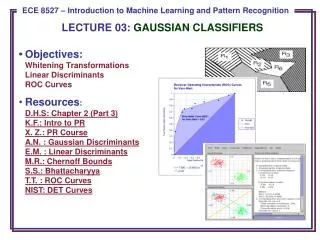
Receiver Operating Characteristic (ROC) • How do we compare two decision rules if they require different thresholds for optimum performance? • Consider four probabilities:
One system can be considered superior to another only if its ROC curve lies above the competing system for the operating region of interest. General ROC Curves • An ROC curve is typically monotonic but not symmetric:
Summary • Decision Surfaces: geometric interpretation of a Bayesian classifier. • Gaussian Distributions: how is the shape of the distribution influenced by the mean and covariance? • Bayesian classifiers for Gaussian distributions: how does the decision surface change as a function of the mean and covariance? • Gaussian Distributions: how is the shape of the decision region influenced by the mean and covariance? • Bounds on performance (i.e., Chernoff, Bhattacharyya) are useful abstractions for obtaining closed-form solutions to problems. • A Receiver Operating Characteristic (ROC) curve is a very useful way to analyze performance and select operating points for systems. • Discrete features can be handled in a way completely analogous to continuous features.
Error Bounds • Bayes decision rule guarantees lowest average error rate • Closed-form solution for two-class Gaussian distributions • Full calculation for high dimensional space difficult • Bounds provide a way to get insight into a problem andengineer better solutions. • Need the following inequality: • Assume a > b without loss of generality: min[a,b] = b. • Also, aβb(1- β) = (a/b)βb and (a/b)β > 1. • Therefore, b < (a/b)βb, which implies min[a,b] < aβb(1- β). • Apply to our standard expression for P(error).
Chernoff Bound • Recall: • Note that this integral is over the entire feature space, not the decision regions (which makes it simpler). • If the conditional probabilities are normal, this expression can be simplified.
where: Chernoff Bound for Normal Densities • If the conditional probabilities are normal, our bound can be evaluated analytically: • Procedure: find the value of β that minimizes exp(-k(β ), and then compute P(error) using the bound. • Benefit: one-dimensional optimization using β
where: Bhattacharyya Bound • The Chernoff bound is loose for extreme values • The Bhattacharyya bound can be derived by β = 0.5: • These bounds can still be used if the distributions are not Gaussian (why? hint: Occam’s Razor). However, they might not be adequately tight.