Orthodox Monetarism
Orthodox Monetarism. Intermediate Macroeconomics ECON-305 Spring 2013 Professor Dalton Boise State University. Purposes. Trace the historical development of modern Monetarism beginning in the 1950s Demand for money Impact of changes in money supply Augmented Phillips Curve

Orthodox Monetarism
E N D
Presentation Transcript
Orthodox Monetarism Intermediate Macroeconomics ECON-305 Spring 2013 Professor Dalton Boise State University
Purposes • Trace the historical development of modern Monetarism beginning in the 1950s • Demand for money • Impact of changes in money supply • Augmented Phillips Curve • Monetary approach to Balance of Payments and Exchange Rates • Summarize the central distinguishing beliefs of Monetarism
Origins of Quantity Theory • Quantity theory of money has been called “the oldest surviving theory in economics” (Blaug) • Many trace it to Locke’s Some Considerations of the Consequences of the Lowering Of Interest and Raising the Value of Money (1692) • Copernicus’s Monetaecudendae ratio (1526) is sometimes afforded the honor • Hume’s Of Money is probably earliest “modern” statement
Origins of Quantity Theory • Martin de AzpilcuetaNavarrus • Comentarioresolutoio de usuras (1556) • first unambiguous statement of quantity theory of money - defines money’s value as its purchasing power, whose value is determined by demand and supply of money • attributed (12 years before Bodin) the price inflation of the mid-16th century to the influx of silver and gold • developed purchasing-power parity theory of exchange rates advanced by colleague Domingo de Soto (1494-1560)
Pre-Keynesian Monetary Theory • Oldest variant is Monetary equilibrium theory • Cambridge k approach • Fisher’s equation of exchange • What is the “quantity theory”? • Confusion with the proportionality theorem (∆M/M = ∆P/P) • Demand and supply theory of monetary value
Quantity Theory in IS-LM • MV = PY • In underemployment conditions V is highly unstable and passively adapts to independent changes in M or PY • Liquidity trap • Interest-inelastic investment • Money demand is unstable and unpredictable
Milton Friedman • Friedman sought to reestablish what he viewed as the Chicago monetary tradition • Series of influential papers and books • Popularization of free market economics Milton Friedman (1912-2006)
Friedman’s Contributions “The Quantity Theory of Money: A Restatement” (1956) “The Supply of Money and Changes in Prices and Output” (1958) “The Demand for Money: Some Theoretical and Empirical Results” (1959) A Monetary History of the United States, 1867-1960 (with Anna Schwartz) (1963)
Friedman’s Contributions “The Relative Stability of Monetary Velocity and the Investment Multiplier in the United States, 1897-1958” (with David Meiselman) (1963) “Interest Rates and the Demand for Money” (1966) “The Role of Monetary Policy” (1968) “A Theoretical Framework for Monetary Analysis” (1970) “Inflation and Unemployment” (1977)
QTM - Money Demand Theory • “The Quantity Theory of Money: A Restatement” (1956) • Money is demanded because it yields a flow of services • Money demand dependent upon • Wealth constraint; Return on money relative to other assets; and, Tastes • In equilibrium, wealth is allocated to equalize marginal return on assets
QTM - Money Demand Theory Md/P = f (rm, rDG, rb, re, þe, h, Yp, u) where rm = return on money, rDG = return on durable goods, rb= return on bonds, re = return on equities, þe = expected inflation rate, h = ratio of income from non-human to human wealth (capital), Yp = permanent income, and u = tastes. Individuals reallocate wealth whenever marginal returns across assets not equal.
Portfolio Adjustment Process Open market purchase of bonds increases Ms Reducing the return on holding money (rm) Money exchanged for financial and real assets Increasing price of equities, price of bonds, price of durable goods (Pe, Pb, PDG) Returns on equities, bonds and durable goods fall (re, rb, rDG) and return on money rises (rm) until equality restored
Portfolio Adjustment Process Conclusions: Broader range of assets and associated expenditures are affected by ∆MS (not just bonds as in Keynes and IS-LM) Stronger, more direct effect on AD due to ∆MS than predicted by Keynes and IS-LM
Money and ∆Nominal Income • Real Money demand changes in stable and predictable ways • V is predictable and stable • Empirical evidence: • Friedman (1959) argued that ∆r do not change Md/P. • Friedman (1966) recanted • No evidence for either liquidity trap or vertical LM curve
Money and ∆Nominal Income • Up to early 1970s money demand was stable (predictable) • Financial innovation of the late 1970s and early 1980s breakdown the stability of Md/P • Relationship between M1 and PY • Regulation Q of Federal Reserve • Clear differentiation between money and not-money
Money and ∆Nominal Income Greenspan: “We don’t know what money is, anymore.”
Role of the Money Supply • “The Supply of Money and Changes in Prices and Output” (1958) • Compared rates of monetary growth with cycle turning points • Peaks (troughs) of monetary growth (∆M/M) preceded peaks (troughs) of cycle by 16 (12) months • Suggestive of monetary influences • Problem of causality
Role of the Money Supply • A Monetary History of the United States, 1867-1960 (with Anna Schwartz) (1963) • Rate of monetary growth slower during contractions than expansions • Negative monetary growth always associated with major contractions • Historical evidence of independent policy changes producing changes in monetary growth • Great Depression consequence of monetary restriction
Role of the Money Supply • “The Relative Stability of Monetary Velocity and the Investment Multiplier in the United States, 1897-1958” (with David Meiselman) (1963) • Compared monetary and Keynesian approaches • ∆C = f(∆Ms) versus ∆C = g(∆I) • Money equation explained more variation in C, except for Great Depression • Poorly conceived
Theoretical Framework • “A Theoretical Framework for Monetary Analysis” (1970) • Until this paper, no explicit formal monetarist model • Friedman intended to show that “the basic differences…are empirical, not theoretical” • Model was IS-LM without Keynesian extremes, without wage rigidity, and with Pigou and real balance effects
Monetarism in mid-1960s 1. Monetary growth predominant factor in explaining nominal income growth. 2. Stable real money demand means economic instability is due to fluctuations in monetary growth induced by monetary authorities. 3. Authorities can control Ms, when they do so, path of nominal income is different than if Ms were endogenous.
Monetarism in mid-1960s 4. Lag between changes in money supply and changes in nominal income is long and variable; discretionary monetary policy is destabilizing. 5. Money supply should grow at a fixed rate of real output growth to stabilize prices.
The 2nd Stage: Phillips Curve Monetary growth is the predominant determinant of nominal income growth and Md is stable and predictable. MV = PY How are changes in Ms divided between P and Y? Augmented Phillips Curve
Augmented Phillips Curve • Friedman, “The Role of Monetary Policy,” AER (1968) • Edmund Phelps, “Phillips Curves, Expectations of Inflation and Optimal Unemployment over Time,” Economica (Aug. 1967) • The original Phillips Curve relationship is misspecified; correcting the misspecification gives a new understanding of the economy.
Augmented Phillips Curve • Original Specification: dW = f(U) • Although W is set in negotiations between employees and employers, both are really interested in w = (W/P). • Inflation (dP) affects w over the contract period. • Inflationary expectations (dPe) therefore affect (dW) • Phillips Curve should be specified as dW = f(U) + dPe.
Augmented Phillips Curve dW PC (dPe2) PC (dPe1) U 5.5% PC (dPe0) Introducing inflationary expectations (dPe) means that rather than one PC there exists a set of Phillips Curves, one for each dPe(where dPe0 < dPe1 < dPe2).
Augmented Phillips Curve LRPC dW PC (dPe2) PC (dPe1) U 5.5% PC (dPe0) There exists a short-run, but NOT a long-run tradeoff between unemployment and inflation. As inflationary expectations adjust to the actual inflation rate, unemployment returns to its natural, full employment, level.
The SR-LR Phillips Curve With zero productivity growth, in equilibrium, dW = dP = dPe. An increase in aggregate demand increases prices, increasing nominal wages. Workers misinterpret the higher nominal wages as higher real wages, given their inflationary expectations, so they increase the quantity of labor they supply. Firms, however, see real wages fall, and are willing to increase employment, reducing unemployment. As workers come to realize that their real wage has fallen, they reduce their labor supply, demanding even higher money wages, reducing employment and increasing unemployment.
A Graphical Presentation SL (Pe1) LRPC SL (Pe0) dW W C W2 B W1 W0 A DL (P1) C B DL (P0) PC (dPe1) A U Lf L1 L 4% 5.5% PC (dPe0)
Augmented Phillips Curve In the short-run, changes in the money supply are non-neutral. In the long-run, once expectations have adjusted, changes in the money supply become neutral.
Empirical Studies • dW = f(U) + ßdPe; assume zero productivity growth • dP = dW; dP = f(U) + ßdPe; equilibium, dP = dPe • dP – ßdP = f(U); dP (1–ß) = f(U) • dP = f(U)/(1-ß) • ß = 1; vertical PC • 0 < ß < 1; neg PC but less favorable • 0 = ß; LRPC and SRPC identical • No clear-cut evidence • Theoretical case overwhelming
Policy Implications 1. Adaptive (Error-learning) expectations imply that U < UN occurs only because of unexpected inflation. 2. Attempts to maintain U < UN only leads to accelerating inflation. 3. Combatting inflation involves output-unemployment costs (U > UN ) and the greater is monetary contraction the greater the costs.
Policy Implications 4. Fixed Rate of Monetary Growth a) Steady monetary growth rate will lead economy to settle at UN. b) Rule removes greatest source of instability. c) Discretionary policy destabilizing due to long and variable lags. d) Because UN not known, policy should not aim at U*.
Policy Implications 5. Permanent reductions in U can only come through removing output and labor restrictions. a) Incentives to work (welfare reform). b) Flexible wages. c) Labor mobility. d) Enterprise privatization.
3rd Stage: Money and BOP • Monetarism and the Balance of Payments • Approach made monetarist analysis relevant to open economies • Fixed Exchange Rates • Currencies are defined as fixed quantities of foreign currencies • Monetary authorities in each country hold reserves of foreign currency (international reserves) to stabilize value of domestic currency relative to foreign currency.
Monetary Approach BOP Fixed Exchange Rates • Key assumptions • Md/P stable function of limited variables • In long run, Y and L tend to YN and LN • In long run, monetary authorities can’t neutralize monetary impact of BOP surpluses or deficits • Arbitrage ensures that prices tend to be equalized
Monetary Approach BOP • Harry Johnson, “The Monetary Approach to Balance of Payments Theory” (1972) • Three Assumptions: Y = YN; law of one price holds in commodity and financial markets; domestic prices and interest rates are pegged to world levels • Md = P* f(Y,r); Ms = D + R, where D equals domestic credit and R equals international reserves • Md = D + R
BOP Analytics What are the effects of increasing domestic credit? Increase D means Ms > Md Individuals rid excess balances by buying foreign goods Generates BOP deficit Authorities sell foreign currency for domestic currency to cover BOP deficit R falls, Ms falls until BOP deficit eliminated ∆D = ∆R
BOP Analytical Dynamics A country experiences persistent BOP deficits and continued loss of international reserves when domestic credit growth (∆D/D) exceeds domestic money demand growth (∆Md/Md) due to real income growth
Policy Implications There exists automatic adjustments to correct BOP disequilibria Discretionary monetary policy is self-defeating Domestic monetary expansion in small open economy has no effect on dP, r, or dY (only foreign reserves) In large open economy, domestic moentary expansion increases world dP
Monetary Approach BOP Flexible Exchange Rates • Frenkel and Johnson, The Economics of Exchange Rates, (1978) • With perfectly flexible exchange rates, exchange rates adjust to clear market so that BOP = 0 • Implies no ∆ in R • Implies ∆D only source of ∆Ms • Therefore, ∆D change ∆Ms and change exchange rates and domestic prices
BOP Analytics What are the effects of increasing domestic credit? Increase D means Ms > Md Individuals rid excess balances by buying foreign goods Excess supply of domestic currency in foreign exchange markets reduces value of domestic currency Depreciation in currency raises domestic prices, increasing Md and money market equilibrium is restored
BOP Analytical Dynamics ε = g(Ms, Y) ∆ε = h(∆Ms, ∆Y) Depreciating exchange rate occurs when domestic monetary growth is faster than domestic real income growth
Orhtodox Monetarism 1. Monetary growth predominant factor in explaining nominal income growth. 2. Economy inherently stable and erratic monetary growth is primary source of economic instability. 3. No long-run tradeoff between inflation and unemployment.
Orthodox Monetarism 4. Prices and BOP are essentially monetary phenomena. 5. Monetary policy should be guided by a rule; fiscal policy should be constrained to traditional roles of distribution and allocation.