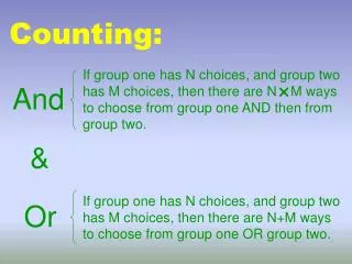
Approximate Counting

1. Approximate Counting SubhasreeBasu Rajiv Ratn Shah Vu Vinh An KiranYedugundla School of Computing National University of Singapore

2. Agenda • Background • The Class #P • Randomized Approximation Schemes • The DNF Counting Problem • Approximating the Permanent • Summary

3. Agenda • Background • The Class #P • Randomized Approximation Schemes • The DNF Counting Problem • Approximating the Permanent • Summary

4. Solvingand Counting • Suppose a problem ∏ • We check if I is an YES-instance of ∏ • That usually involves finding the solution to ∏ and checking if I matches it

5. Example If we want to find all possible permutations of 3 different items

6. Example If we want to find all possible permutations of 3 different items

7. Solving and Counting • When we are trying to count, we actually try to find the number of solutions of ∏ where I is a solution • Following the same example, in the counting version we want to know how many such permutations exist

8. Approximate Counting • Approximate Counting – involves two terms Approximate and Counting • Counting is getting the number of solutions to a problem • Approximate because we do not have an exact counting formula for a vast class of problems Approximately counting Hamilton paths and cycles in dense graphsMartin Dyer, Alan Frieze, and Mark Jerrum, SIAM Journal on Computing27 (1998), 1262-1272.

9. Agenda • Background • The Class #P • Randomized Approximation Schemes • The DNF Counting Problem • Approximating the Permanent • Summary

10. The Class #P • #P is the class of counting problems associated with the NP decision problems • Formally a problem ∏ belongs to the #P if there is a non-deterministic polynomial time Turing Machine that, for any instance I, has a number of accepting computations that is exactly equal to the number of distinct solutions to instance I • ∏ is #P-complete if for any problem ∏’ in #P, ∏’ can be reduced to ∏ by a polynomial time Turing machine.

11. Need for Randomization • #P-complete problems can only be solvable in polynomial time only if P=NP • Hence the need for approximate solutions • Randomization is one such technique to find approximate answers to counting problems

12. Various Applications for Approximate Counting • DNF counting problem. • Network reliability. • Counting the number of Knapsack solutions. • Approximating the Permanent. • Estimating the volume of a convex body.

13. Various Applications for Approximate Counting • DNF counting problem. • Network reliability. • Counting the number of Knapsack solutions. • Approximating the Permanent. • Estimating the volume of a convex body.

14. Agenda • Background • The Class #P • Randomized Approximation Schemes • The DNF Counting Problem • Approximating the Permanent • Summary

15. Polynomial Approximation Scheme • Let #(I) be the number of distinct solutions for instance I of problem ∏ • Let the Approximation algorithm be called A • It takes an input I and outputs and integer A(I) • A(I) is supposed to be close to #(I)

16. Polynomial Approximation Scheme DEF 1: A Polynomial Approximation scheme(PAS) for a counting problem is a deterministic algorithm A that takes and input instance I and a real number ε > 0, and in time polynomial in n = |I| produces an output A(I) such that (1- ε) #(I) < A(I) < (1 + ε) #(I)

17. Polynomial Approximation Scheme DEF 1: A polynomial Approximation scheme(PAS) for a counting problem is a deterministic algorithm A that takes and input instance I and a real number ε > 0, and in time polynomial in n = |I| produces an ouput A(I) such that (1- ε) #(I) < A(I) < (1 + ε) #(I) DEF 2 :A Fully Polynomial Approximation Scheme (FPAS) is a polynomial approximation scheme whose running time is polynomially bounded in both n and 1/ε. The output A(I) is called an ε-approximation to #(I)

18. Polynomial Randomized Approximation Algorithm DEF 3: A Polynomial Randomized Approximation scheme(PRAS) for a counting problem ∏ is a randomized algorithm A that takes an input instance I and a real number ε>0, and in time polynomial in n = |I| produces an output A(I) such that Pr[(1- ε)#(I) ≤ A(I) ≤ (1 + ε)#(I)] ≥ ¾

19. Polynomial Randomized Approximation Algorithm DEF 3: A Polynomial Randomized Approximation scheme(PRAS) for a counting problem ∏ is a randomized algorithm A that takes an input instance I and a real number ε>0, and in time polynomial in n = |I| produces an output A(I) such that Pr[(1- ε)#(I) ≤ A(I) ≤ (1 + ε)#(I)] ≥ 3/4 DEF 4: A Fully Polynomial Randomized Approximation Scheme (FPRAS) is a polynomial randomized approximation scheme whose running time is polynomially bounded in both n and 1/ε.

20. An (ε, δ) FPRAS DEF 5: An (ε, δ)-FPRAS for a counting problem ∏ is a fully polynomial randomized approximation scheme that takes an input instance I and computes an ε-approximation to #(I) with probability at least 1- δ in time polynomial in n , 1/ εand log(1/δ)

21. Agenda • Background • The Class #P • Randomized Approximation Schemes • The DNF Counting Problem • Approximating the Permanent • Summary

22. Monte Carlo Method • It is a wide-range of algorithms under one name • In essence it includes all the techniques that use random numbers to simulate a problem • It owes its name to a casino in the principality of Monte Carlo. • Events in a casino depend heavily on chance of a random event. e.g., ball falling into a particular slot on a roulette wheel, being dealt useful cards from a randomly shuffled deck, or the dice falling the right way

23. DNF Counting - Terminologies • F(X1, X2,… Xn) is Boolean formula in DNF • X1, X2,… Xn are Boolean variables. • F = C1 ∨ C2… ∨ Cm is a disjunction of clauses • Ci= L1 ∧ L2… ∧ Lriis a conjunction of Literals • Li is either variable Xk or Xk’ e.g. F = (x1 ∧ x3’) ∨ (x1 ∧ x2’∧ x3) ∨ (x2 ∧ x3)

24. Terminologies contd … • a = (a1, a2, … an ) is truth assignment • a satisfy F if F(a1, a2, … an ) evaluates to 1 or TRUE • #F is the number of distinct satisfying assignment of F Clearly we have here 0 < #F ≤ 2n

25. DNF Counting Problem • The Problem at hand is now to compute the value of #F • It is known to be #P complete (We can reduce #SAT to #P complete) • We will describe an (ε, δ)- FPRAS algorithm for this • The input size for this is at most nm • We have to design a approximation scheme that has a running time polynomial in n, m , 1/ εand log(1/ δ)

26. Some more terminologies • U is a finite set of known size • f: U {0,1} be a Boolean function over U • Define G = {u є U | f(u) =1} as the pre-image of U Assume: we can sample uniformly at random from U We now want to find the size of G i.e., |G|

27. Formulation of Our Problem • Let in our formulation U = {0,1}n , the set of all 2n truth assignments • Let f(a) = F(a) for each of aєU • Hence our G is now the set of all satisfying truth assignments for F Our problem thus reduces to finding the size of G

28. Monte Carlo method • Choose N independent samples from U, say, u1, u2, ……. ,uN • Use the value of f on these samples to estimate the probability that a random choice will lie in G • Define the random variable Yi = 1 if f(ui) =1 , Yi = 0 otherwise So Yi is 1 if and only if uiєG • The estimator random variable is Z = |U| We claim that with high probability Z will be an approximation to |G|

29. An Unsuccessful Attempt (cont.) • Estimator Theorem: Let ρ = , Then Monte Carlo method yields an -approximation to |G| with probability at least 1 – δ provided N ≥ • Why unsuccessful? • We don’t know the value of ρ • We can solve this by using a successively refined lower bound on to determine the number of samples to be chosen • It has running time of at least N. where N ≥

30. Agenda • Background • Randomized Approximation Schemes • The DNF Counting Problem • DNF Counting • Compute #F • An Unsuccessful Attempt • The Coverage Algorithm • Approximating the Permanent • Summary

31. DNF Counting • Let F = C1∨ C2∨ C3∨ C4 = (x1 ∧ x3’) ∨ (x1 ∧ x2’∧ x3) ∨ (x2 ∧ x3) ∨ (x3’) • G be set of all satisfying truth assignment • Hi be set of all satisfying truth assignment for Ci • H1 = {a5, a7} • H2 = {a6} • H3 = {a4, a8} • H4 = {a1, a3, a5, a7} • H = H1 H2 H3 H4 = {a1, a3, a4, a5, a6, a7, a8} • It is easy to see that |Hi | = 2 n-ri H2 H4 H3 H1

32. DNF Counting |G| = #F a1 a2 . . ai aj . . . . a2n 0 , f(a) = F(a) f: V→ {0, 1} 1 V

33. The Coverage Algorithm • Importance Sampling • Want to reduce the size of the sample space • Ratio ρ is relatively large • Ensuring that the set G is still completely represented. • Reformulate the DNF counting problem in a more abstract framework, called the union of sets problem.

34. union of sets problem • union of setsproblem Let V be a finite Universe. We are given m subsets H1, H2, …, Hm ⊆ V, such that following assumptions are valid: • For all i, |Hi| is computable in polynomial time. • It is possible to sample uniformly at random from any Hi • For all v ∈ V, it can be determined in polynomial time whether v ∈ Hi • The Goal is to estimate the size of the Union H = H1 ∪ H2 ∪ … ∪ Hm • The brute-force approach to compute |H| is inefficient when the universe and the set Hi are of large cardinality • The assumption 1-3 turn out to be sufficient to enable the design of Importance sampling algorithm

35. DNF Counting . . . . . . . . Hi 0, H1 H2 1 Hm F[v] → {0, 1} V

36. The Coverage Algorithm • DNF Counting is special case of union of sets • F(X1, X2,… Xn) is Boolean formula in DNF • The universe V corresponds to the space of all 2n truth assignment • Set Hi contains all the truth assignment that satisfy the clause Ci • Easy to sample from Hi by assigning appropriate values to variables appearing in Ciand choosing rest at random • Easy to see that |Hi | = 2 n-ri • Verify in linear timethat some v ∈ V is a member of Hi • Then the union of sets Hi gives the set of satisfying assignments for F

37. The Coverage Algorithm • Solution to union of sets problem. • Define a multiset U = H1 ⊎ H2 … ⊎ Hm • Multiset union contains as many copies of v ∈ V as the number of Hi`sthat contain that v. • U = {(v,i) | (v,i)∈ Hi} • Observe that |U| = ≥ |H| • For all v ∈ H, cov(v) = {(v,i) | (v,i) ∈ U} • In DNF problem, for a truth assignment a, the set cov(a) is the set of clauses satisfied by a

38. The Coverage Algorithm • The following observations are immediate • The number of coverage set is exactly |H| • U = COV(v) • |U| = • For all v ∈ H, |COV(v)| ≤ m • Define function f((v, i)) = {1 if i = min{ j |v j}; 0 otherwise} • Define set G = {(v, i) U | f((v, i)) = 1} • |G| = |H|

39. The Coverage Algorithm • Algorithm • for j = 1 to N do • pick (v, i) uniformly at random from U • Set Yj =1 if f((v, i)) = 1 ; else 0 // if((v, i)) = 1, call it special pair • Output().|U| = Y .|U| • E[Yj] = = = = • So the algorithm is an unbiased estimator for as desired R.M. Karp and M. Luby, “Monte-carlo algorithms for enumeration and reliability problems,” In Proceedings of the 15th Annual ACM Symposium on Theory of Computing, 1983, pp. 56–64.

40. Analysis • The Value of N: • E[Yj] = ≥ = • By Estimator Theorem N = = # trials • Complexity • Computing |U| requires O(nm) • Checking (v, i) is special requires O(nm) • Generating a random pair requires O(n+m) • Total running time per trial = O(nm) • Total running time = O() Karp, R., Luby, M., Madras, N., “Monte-Carlo Approximation Algorithms for Enumeration Problems", J. of Algorithms, Vol. 10, No. 3, Sept. 1989, pp. 429-448. improved the running time to O()

41. (, δ)-FPRAS for DNF Counting • Our Goal is to estimate the size of G ⊆ U such that G = f-1(1) • Apply Estimator Theorem based on naïve Monte Carlo sampling technique We claim that the naïve Monte Carlo sampling algorithm gives an (, δ)-FPRAS for estimating the size of G. Lemma: In the union of sets problem ρ = Proof: relies on the observations made above • |U| = ≤ ≤ m|H| = m|G|

42. The Coverage Algorithm • The Monte Carlo Sampling technique gives as (, δ)-FPRAS for |G|, hence also for |H| Estimator Theorem:The Monte Carlo method yields an -approximation to |G| with probability at least 1 - δ provided N ≥ The running time is polynomial in N Proof: We need to show: • fcan be calculated in polynomial time • It is possible to sample uniformly from U.

43. The Coverage Algorithm Proof(1): Compute f((v,i)) in O(mn) by checking whether truth assignment v satisfies Ci but none of the clauses Cj for j <i. Proof(2): It is possible to sample uniformly from U. Sampling an element (v,i) uniformly from U: • choose is.t. 1 ≤ i ≤ m and Pr[i] = = = • Set the Variables in Hi so that Hi is satisfied • choose a truth assignment for the remaining variables uniformly at random • output iand the resulting truth assignment v

44. Agenda • Background • Randomized Approximation Schemes • The DNF Counting Problem • Approximating the Permanent • Number of perfect matchings in bipartite graph • Near-uniform generation • The canonical path argument • Summary

45. Matrix Permanent • The permanent of a square matrix in linear algebra is a function of the matrix similar to the determinant. The permanent, as well as the determinant, is a polynomial in the entries of the matrix. • Permanent formula: Let be an matrix, the permanent of the matrix is defined as: Where • Example: • Best running time: A Z Broder. 1986. How hard is it to marry at random? (On the approximation of the permanent). In Proceedings of the eighteenth annual ACM symposium on Theory of computing (STOC '86). ACM, New York, NY, USA, 50-58. DOI=10.1145/12130.12136

46. Agenda • Background • Randomized Approximation Schemes • The DNF Counting Problem • Approximating the Permanent • Number of perfect matchings in bipartite graph • Near-uniform generation • The canonical path argument • Summary

47. Bipartite Graph • Definition: a bipartite graph is a set of graph vertices decomposed into two disjoint sets such that no two graph vertices within the same set are adjacent. • Notations: G(U, V, E) where: • are disjoint sets of vertices in which n is number of vertices in each set • E is set of graph edges • Bipartite graph G could be represented in 0-1 matrix A(G) as following: U1 V1 V2 V1 U1 U2 V2 U2

48. Graph Perfect Matchings • A matching is a collection of edges such that vertex occurs at most once in M • A perfect matching is a matching of size n U1 V1 U1 V1 U2 V2 U2 V2 Rajeev Motwani and PrabhakarRaghavan. 1995. Randomized Algorithms. Cambridge University Press, New York, NY, USA. Chapter 11.

49. Graph Perfect Matchings • Let denote the number of perfect matchings in the bipartite graph G: • Computing the number of perfect matchings in a given bipartite graph is #P-complete  computing permanent of 0-1 matrix is also #P-complete • Propose a for counting number of perfect matchings problem V2 V1 U1 V1 U1 U2 U2 V2

50. Introduction to Monte Carlo Method • A method which solves a problem by generating suitable random numbers and observing that fraction of the numbers obeying some properties • Monte Carlo methods tend to follow a particular pattern: • Define a domain of possible inputs. • Generate inputs randomly from a probability distribution over the domain. • Perform a deterministic computation on the inputs. • Aggregate the results.