Cross Layer Adaptive Control for Wireless Mesh Networks
240 likes | 265 Vues
Explore cross-layer networking strategies to optimize wireless mesh network performance. Understand instantaneous capacity regions and design algorithms for throughput and delay efficiency.

Cross Layer Adaptive Control for Wireless Mesh Networks
E N D
Presentation Transcript
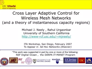
Cross Layer Adaptive Control for Wireless Mesh Networks (and a theory of instantaneous capacity regions) Michael J. Neely , Rahul Urgaonkar University of Southern California http://www-rcf.usc.edu/~mjneely/ ITA Workshop, San Diego, February 2007 To Appear in Ad Hoc Networks (Elsevier) *This work was supported in part by one or more of the following: NSF Digital Ocean , the DARPA IT-MANET Program
Cross Layer Networking Network Layering Timescale Decomposition Transport “Flow Control” Flow/Session Arrival and Departure Timescales Network “Routing” Mobility Timescales PHY/MAC “Resource Allocation” “Scheduling” Channel Fading Channel Measurement Objective: Design Algs. for Throughput and Delay Efficiency Fact: Network Performance Limits are different across different layers and timescales Example…
Mobile Network at Different Timescales “Ergodic Capacity” -Thruput = O(1) -Connectivity Graph is 2-Hop (Grossglauser-Tse) “Capacity and Delay Tradeoffs” -Neely, Modiano [2003, 2005] -Shah et. al. [2004, 2006] -Toumpis, Goldsmith [2004] -Lin, Shroff [2004] -Sharma, Mazumdar, Shroff [2006]
Mobile Network at Different Timescales “Instantaneous Capacity” -Thruput = O(1/sqrt{N}) -Connectivity Graph for a “snapshot” in time -Thruput can be much larger if only a few sources are active at any one time!
Mobile Network at Different Timescales “Instantaneous Capacity” -Thruput = O(1/sqrt{N}) -Connectivity Graph for a “snapshot” in time -Thruput can be much larger if only a few sources are active at any one time!
lij Network Model --- The General Picture Flow Control Decision Rij(t) own other 3 Layers: • Flow Control (Transport) • Routing (Network) • Resource Alloc./Sched. (MAC/PHY) *From: Resource Allocation and Cross-Layer Control in Wireless Networks by Georgiadis, Neely, Tassiulas, NOW Foundations and Trends in Networking, 2006
Network Model --- The General Picture own other 3 Layers: Flow Control (Transport) Routing (Network) Resource Alloc./Sched. (MAC/PHY) *From: Resource Allocation and Cross-Layer Control in Wireless Networks by Georgiadis, Neely, Tassiulas, NOW Foundations and Trends in Networking, 2006
Network Model --- The General Picture own other “Data Pumping Capabilities”: (mij(t)) = C(I(t), S(t)) Control Action (Resource Allocation/Power) Channel State Matrix 3 Layers: Flow Control (Transport) Routing (Network) Resource Alloc./Sched. (MAC/PHY) I(t) in I *From: Resource Allocation and Cross-Layer Control in Wireless Networks by Georgiadis, Neely, Tassiulas, NOW Foundations and Trends in Networking, 2006
Network Model --- The Wireless Mesh Architecture with Cell Regions Mesh Clients: -Mobile -Peak and Avg. Power Constrained (Ppeak, Pav) -Little/no knowledge of network topology Mesh Routers: -Stationary (1 per cell) -More powerful/knowedgeable -Facillitate Routing for Clients 1 2 8 7 4 0 6 3 5 9 Assume Slotted Time t in {0, 1, 2, …} Let T(t) = Topology State of Clients on slot t (Arbitrary Mobility) Let S(t) = Channel States of Links on slot t Assume: S(t) is conditionally i.i.d. given T(t): pS(T) = Pr[S(t) = S | T(t)=T ]
Instantaneous Capacity Region The Instantaneous Capacity Region: 1 2 8 7 4 0 6 3 5 L(t) = Instantaneous Capacity Region = Ergodic Capacity Associated with a network with fixed topology state T(t) for all time (and i.i.d. channels pS(T)) 9 Assume Slotted Time t in {0, 1, 2, …} Let T(t) = Topology State of Clients on slot t (Arbitrary Mobility) Let S(t) = Channel States of Links on slot t Assume: S(t) is conditionally i.i.d. given T(t): pS(T) = Pr[S(t) = S | T(t)=T ]
Instantaneous Capacity Region The Instantaneous Capacity Region: 1 2 8 7 4 0 6 3 5 L(t) = Instantaneous Capacity Region = Ergodic Capacity Associated with a network with fixed topology state T(t) for all time (and i.i.d. channels pS(T)) 9 Assume Slotted Time t in {0, 1, 2, …} Let T(t) = Topology State of Clients on slot t (Arbitrary Mobility) Let S(t) = Channel States of Links on slot t Assume: S(t) is conditionally i.i.d. given T(t): pS(T) = Pr[S(t) = S | T(t)=T ]
Instantaneous Capacity Region The Instantaneous Capacity Region: 1 2 8 7 4 0 6 3 5 L(t) = Instantaneous Capacity Region = Ergodic Capacity Associated with a network with fixed topology state T(t) for all time (and i.i.d. channels pS(T)) 9 Assume Slotted Time t in {0, 1, 2, …} Let T(t) = Topology State of Clients on slot t (Arbitrary Mobility) Let S(t) = Channel States of Links on slot t Assume: S(t) is conditionally i.i.d. given T(t): pS(T) = Pr[S(t) = S | T(t)=T ]
Instantaneous Capacity Region The Instantaneous Capacity Region: 1 2 8 7 4 0 6 3 5 L(t) = Instantaneous Capacity Region = Ergodic Capacity Associated with a network with fixed topology state T(t) for all time (and i.i.d. channels pS(T)) 9 Assume Slotted Time t in {0, 1, 2, …} Let T(t) = Topology State of Clients on slot t (Arbitrary Mobility) Let S(t) = Channel States of Links on slot t Assume: S(t) is conditionally i.i.d. given T(t): pS(T) = Pr[S(t) = S | T(t)=T ]
Instantaneous Capacity Region The Instantaneous Capacity Region: 2 1 8 7 0 6 4 3 5 L(t) = Instantaneous Capacity Region = Ergodic Capacity Associated with a network with fixed topology state T(t) for all time (and i.i.d. channels pS(T)) 9 Assume Slotted Time t in {0, 1, 2, …} Let T(t) = Topology State of Clients on slot t (Arbitrary Mobility) Let S(t) = Channel States of Links on slot t Assume: S(t) is conditionally i.i.d. given T(t): pS(T) = Pr[S(t) = S | T(t)=T ]
Instantaneous Capacity Region The Instantaneous Capacity Region: 2 1 8 7 0 6 4 3 5 L(t) = Instantaneous Capacity Region = Ergodic Capacity Associated with a network with fixed topology state T(t) for all time (and i.i.d. channels pS(T)) 9 Assume Slotted Time t in {0, 1, 2, …} Let T(t) = Topology State of Clients on slot t (Arbitrary Mobility) Let S(t) = Channel States of Links on slot t Assume: S(t) is conditionally i.i.d. given T(t): pS(T) = Pr[S(t) = S | T(t)=T ]
Instantaneous Capacity Region The Instantaneous Capacity Region: 2 1 8 7 0 4 3 6 5 L(t) = Instantaneous Capacity Region = Ergodic Capacity Associated with a network with fixed topology state T(t) for all time (and i.i.d. channels pS(T)) 9 Assume Slotted Time t in {0, 1, 2, …} Let T(t) = Topology State of Clients on slot t (Arbitrary Mobility) Let S(t) = Channel States of Links on slot t Assume: S(t) is conditionally i.i.d. given T(t): pS(T) = Pr[S(t) = S | T(t)=T ]
Results: -Design a Cross-Layer Algorithm that optimizes throughput-utility with delay that is independent of timescales of mobility processT(t). -Use *Lyapunov Network Optimization -Algorithm Continuously Adapts *[Tassiulas, Ephremides 1992] (Backpressure, MWM) *[Georgiadis, Neely, Tassiulas F&T 2006] *[Neely, Modiano, 2003, 2005] T2 T1 T3 } (Stochastic Network Optimization)
Algorithm: (CLC-Mesh) Utility-Based Distributed Flow Control for Stochastic Nets -gi(x) = concave utility (ex: gi(x) = log(1 + x)) -Flow Control Parameter V affects utility optimization / max buffer size tradeoff x = thruput Combined Backpressure Routing/Scheduling with “Estimated” Shortest Path Routing at Mesh Routers -Mesh Router Nodes keep a running estimate of client locations (can be out of date) -Use Differential Backlog Concepts -Use a Modified Differential Backlog Weight that incorporates: (i) Shortest Path Estimate (ii) Guaranteed max buffer size hV (provides immediate avg. delay bound) -Virtual Power Queues for Avg. Power Constraints [Neely 2005]
Define: g*(t) = Optimal Utility Subject to Instantaneous Capacity Region Instantaneous Capacity Region L(t1) Instantaneous Capacity Region L(t2) Instantaneous utility-optimal point Instantaneous utility-optimal point Theorem: Under CLC-Mesh with flow control parameter V, we have: Backlog: Ui(t) <= hV for all time t (worst case buffer size in all network queues) Peak and Average Power Constraints satisfied at Clients (c)
Define: g*(t) = Optimal Utility Subject to Instantaneous Capacity Region Instantaneous Capacity Region L(t1) Instantaneous Capacity Region L(t2) Instantaneous utility-optimal point Instantaneous utility-optimal point e Theorem: Under CLC-Mesh with flow control parameter V, we have: (d) If V = infinity (no flow control) and rate vector is always interior to instantaneous capacity region (distance at most e from boundary), then achieve 100% throughput with delay that is independent of mobility timescales. (e) If V = infinity (no flow control), if mobility process is ergodic, and rate vector is inside the ergodic capacity region, then achieve 100% throughput with same algorithm, but with delay that is on the order of the “mixing times” of the mobility process.
Simulation Experiment 1 10 Mesh clients, 21 Mesh Routers in a cell-partitioned network Communication pairs: 0 1, 2 3, …, 8 9 0 1 2 8 7 4 6 3 5 9 Halfway through the simulation, node 0 moves (non-ergodically) from its initial location to its final location. Node 9 takes a Markov Random walk. Full throughput is maintained throughout, with noticeable delay increase (at “new equilibrium”), but which is independent of mobility timescales.
Simulation Experiment 2 Flow control using control parameter V • The achieved throughput is very close to the input rate for small values • of the input rate • The achieved throughput saturates at a value determined by the V • parameter, being very close to the network capacity (shown as vertical • asymptote) for large V
Simulation Experiment 3 Effectiveness of Combined Diff. Backlog -Shortest Path Metric
Simulation Experiment 3 Effectiveness of Combined Diff. Backlog -Shortest Path Metric Interpretation of this slide: Omega = weight determining degree to which shortest path estimate is used. Omega = 0 means pure differential backlog (no shortest path estimate) Full Thruput is maintained for any Omega (Omega only affects delay for low input rates)