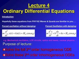
Lecture 4 Ordinary Differential Equations

1. Lecture 4Ordinary Differential Equations Purpose of lecture: • Solve the full 2nd order homogeneous ODE • Solve these 2nd order inhomogeneous ODEs Introduction Hopefully these equations from PHY102 Waves & Quanta are familiar to you…. Forced oscillation without damping: Forced Oscillation with damping: e.g. Mechanical oscillators, LCR circuits, optics and lasers, nuclear physics, …

2. 2nd order homogeneous ODE Solving Step 1: Let the trial solution be Now substitute this back into the ODE remembering that and This is now called the auxiliary equation Step 2: Solve the auxiliary equation for and Step 3: General solution is or if m1=m2 For complex roots solution is which is same as or Step 4: Particular solution is found now by applying boundary conditions

3. Step 1: Trial solution is so auxiliary equation Step 2: Solving the auxiliary equation gives Step 3: General solution is if m1=m2 giving Step 4: Particular solution is found now by applying boundary conditions When t = 0, x = 4 so and so Since velocity = Boundary conditions give so Full solution is therefore 2nd order homogeneous ODE Solve Boundary conditions x=4, velocity=0 when t=0

4. 2nd order homogeneous ODE Example 3: Damped harmonic oscillators Effect of damper drag will be a function of Rally suspension http://uk.youtube.com/watch?v=CZeCuS4xzL0&feature=related 4x4 with no shock absorbers http://uk.youtube.com/watch?v=AKcTA5j6K80&feature=related Bose suspension http://uk.youtube.com/watch?v=eSi6J-QK1lw Crosswind landing http://uk.youtube.com/watch?v=n9yF09DMrrI

5. 2nd order homogeneous ODE Example 3: Linear harmonic oscillator with damping Step 1: Let the trial solution be So and Step 2: The auxiliary is then with roots Step 3: General solution is then……. HANG ON!!!!! In the last lecture we determined the relationship between x and t when meaning that will always be real What if or ???????????????????

6. 2nd order homogeneous ODE Example 3: Damped harmonic oscillator Auxiliary is roots are BE CAREFUL – THERE ARE THREE DIFFERENT CASES!!!!! (i) Over-damped gives two real roots Both m1and m2are negative so x(t) is the sum of two exponential decay terms and so tends pretty quickly, to zero. The effect of the spring has been made of secondary importance to the huge damping, e.g. aircraft suspension

7. 2nd order homogeneous ODE Example 3: Damped harmonic oscillator Auxiliary is roots are BE CAREFUL – THERE ARE THREE DIFFERENT CASES!!!!! (ii) Critically damped gives a single root Here the damping has been reduced a little so the spring can act to change the displacement quicker. However the damping is still high enough that the displacement does not pass through the equilibrium position, e.g. car suspension.

8. (iii) Under-damped This will yield complex solutions due to presence of square root of a negative number. Let so thus As before general solution with complex roots can be written as The solution is the product of a sinusoidal term and an exponential decay term – so represents sinusoidal oscillations of decreasing amplitude. E.g. bed springs. 2nd order homogeneous ODE Example 3: Damped harmonic oscillator Auxiliary is roots are BE CAREFUL – THERE ARE THREE DIFFERENT CASES!!!!! We do this so that W is real

9. 2nd order homogeneous ODE Example 3: Damped harmonic oscillator Auxiliary is roots are BE CAREFUL – THERE ARE THREE DIFFERENT CASES!!!!! Q factor A high Q factor means the oscillations will die more slowly

10. Inhomogeneous ordinary differential equations Step 1: Find the general solution to the related homogeneous equation and call it the complementary solution . Step 2: Find the particular solution of the equation by substituting an appropriate trial solution into the full original inhomogeneous ODE. e.g. If f(t) = t2try xp(t) = at2 + bt + c If f(t) = 5e3ttry xp(t) = ae3t If f(t) = 5eiωt try xp(t) =aeiωt If f(t) = sin2t try xp(t) = a(cos2t) + b(sin2t) If f(t) = cos wt try xp(t) =Re[aeiωt] see later for explanation If f(t) = sin wt try xp(t) =Im[aeiωt] If your trial solution has the correct form, substituting it into the differential equation will yield the values of the constants a, b, c, etc. Step 3: The complete general solution is then . Step 4: Apply boundary conditions to find the values of the constants

11. Inhomogeneous ODEs Step 1: The corresponding homogeneous general equation is the LHO that we solved in last lecture, therefore Step 2: For we should use trial solution Putting this into FULL ODE gives:- Comparing terms we can say that b = 0 and So Step 3: So full solution is Example 4: Undamped driven oscillator At rest when t = 0 and x = L

12. Inhomogeneous ordinary differential equations When t = 0, x = L so At rest means velocity at x = L and t = 0. So differentiate full solution and as velocity = 0 when t = 0 so Full solution is therefore Example 4: Undamped driven oscillator At rest when t = 0 and x = L Step 4: Apply boundary conditions to find the values of the constants for the full solution

13. Undamped driven oscillator with SHM driving force This can also be written as • A few comments • Note that the solution is clearly not valid for • The ratio is sometimes called the response of the • oscillator. It is a function of w. It is positive for w < w0, negative for w > w0 . This means that at low frequency the oscillator follows the driving force but at high frequencies it is always going in the ‘wrong’ direction. • ! The ratio