Download

1 / 73
730 likes | 914 Vues
Numerical Techniques of Natural Circulation: History and Background Juan Carlos Ferreri Autoridad Regulatoria Nuclear, Buenos Aires, Argentina Course on Natural Circulation Phenomena and Modelling in Water-cooled Nuclear Reactors ICTP, Trieste, Italy, 25 to 29 June, 2007. CONTENTS

E N D
Numerical Techniques of Natural Circulation: History and Background Juan Carlos FerreriAutoridad Regulatoria Nuclear, Buenos Aires, ArgentinaCourse on Natural Circulation Phenomena and Modelling in Water-cooled Nuclear ReactorsICTP, Trieste, Italy, 25 to 29 June, 2007
CONTENTS • Purpose of this presentation and introductory remarks • On numerical methods • A brief review of present status of CFD in relation to natural circulation, best practices and other issues • Conclusions
This presentation is aimed at considering several aspects of Numerical Techniques giving the background to the computation of Fluid Dynamics as applied to the Computational Fluid Dynamics (CFD) of Natural Circulation (NC). It will be shown that: • There is plenty of consolidated literature and concepts on numerical methods since 50 years ago. • CFD is not a new activity in relation to NC and the thermal hydraulics of Nuclear Safety • Many outstanding people contributed to this subject in the last five decades PURPOSE OF THIS PRESENTATION
The present boom of CFD activity in NC and on separate effects in nuclear installations is a consequence of the needs of a re-emerging activity • Nuclear Safety benefits from well developed techniques in other areas of computational mechanics • Although some spectacular CFD results may be found at TH fora and in open (www) sources, not so many are already published in regular journals. • Most publications deal with the needs and challenges posed by the physics and with clarifying the degree of detail required by nuclear safety PURPOSE OF THIS PRESENTATION
Two possible definitions in this context: • A numerical technique is an incremental (or discrete) way of representing a differential equation (that is part of a physical model in NC) • Computational Fluid Dynamics is a discipline that allows solving conservation equations using adequate discrete representations at a desired level of resolution, implying more than a numerical technique INTRODUCTORY REMARKS
On pioneers… Obviously, numerical techniques applications are not a new activity in relation to the thermal hydraulics of all the flow stages of transients in nuclear installations (NC among others). In my view, it was the work at Los Alamos Scientific Laboratory which (now more than 30 years ago), in those days of “open” exchange of scientific information, opened the way to “widespread” numerical modeling in fluid dynamics. See, e.g.: Los Alamos Science, vol. 2, no. 2, summer/fall 1981 summarizing work done up to that year at LANL INTRODUCTORY REMARKS
People, people… Many outstanding people contributed to this activity in the last 50 years... However, again in my view, LANL pioneered in this subject and its most relevant people were: Francis H. Harlow, J. Fromm, C.W. Hirt, D.L. Liles, J. Mahaffy, A.A. Amsdem, J.R. Travis, J.P. Shanon, J. Pryor and B.J. Daly, among others. Perhaps you have heard about codes like PIC, SOLA, SOLA-SURF, SOLA-DF, SOLA-VOF, SALE-3D, SOLALOOP, K-FIX, etc. (see J.Comp. Physics) P. Roache gave also an important and comprehensive review and recommendations on numerical techniques and CFD by 1972. People at LLNL also contributed significantly INTRODUCTORY REMARKS
People, people… Other people pioneered in Europe, like B. Spalding, M. Wolfshtein, S. Patankar at Imperial College, R. Peiret at ONERA and many others. I will just mention some people that contributed to the development from the numerical analysis side... …because the list is too long, but the names of R. Courant, K.O. Friedrichs, D. Hilbert, J. von Neumann, P.D. Lax, R.D. Richtmyer, G.I. Marchuk (in Russia) and W.F. Ames should, at least, be mentioned. INTRODUCTORY REMARKS
People, people… The Drift-Flux theory of two-phase flow, as developed by Zuber and Findlay and by M. Ishii in his book, was the physical two-phase fluid model that allowed generating results of Nuclear Safety significance through its implementation in the TRAC code and other hydrodynamics codes at LASL. Many other people contributed significantly in this field, like J.M. Delhaye, R. Lahey, M. Giot, F.H Moody, G.B. Wallis, R.E. Henry, J.A. Bouré, D.C. Groeneveld, G. Yadigaroglu and simply too many others to be cited here… INTRODUCTORY REMARKS
An appropriate conceptual excerpt… • “In as much as we can simulate reality, we can use the computer to make predictions about what will occur in a certain set of circumstances. • Finite-difference techniques can create an artificial laboratory for examining situations which would be impossible to observe otherwise, but we must always remain critical of our results. • Finite-differencing can be an extremely powerful tool, but only when it is firmly set in a basis of physical meaning. In order for a finite-difference code to be successful, we must start from the beginning, dealing with simple cases and examining our logic each step of the way.” Reference: E. Scannapieco and Francis H. Harlow, Introduction to Finite-Difference Methods for Numerical Fluid Dynamics, LA 12984, issued 1995 INTRODUCTORY REMARKS
Some examples i.e. 13500 computing cellscode: SALE-3D “Detailed studies of reactor components”, A.A. Amsdem et al., Los Alamos Science, 1981, pp. 54-73 INTRODUCTORY REMARKS
Some examples 1331 fluid computing cells code: a SOLA 3D like… With far more modest resources we were working too… B. Martinez and J.C. Ferreri, Lat. American J. of Heat and Mass Transfer, vol. 6, pp. 1-12, 1982and other references before… INTRODUCTORY REMARKS
A proposal for what follows… Understanding the need of making efforts in the appropriate modelling of 1D flows fluid dynamics (this seems a somewhat old-fashioned proposal at this time, when multi-dimensional CFD modelling governs the trends in the analysis of NC and separate effects in Nuclear Safety related issues) However, let´s make... INTRODUCTORY REMARKS
For single-phase flows in vertical pipes (or two-phase flows with equal velocities and temperature), the effects of each term in the conservation equations are preserved in model and prototype without any distortion, if one imposes the requirements of: a) Same fluid at equal pressure, properties and enthalpy: b) Isochronous phenomena: They lead to the Power to Volume scaling relations, i.e.: Where m is chosen on the basis of available resources, usually power for the model Reference: N. Zuber, "Problems in Modeling of Small Break LOCA", NUREG-0724, 1980 A small digression on scaling laws… INTRODUCTORY REMARKS
c) Imposing now equal elevations: (This condition is essential to keep equal gravity driving forces, i.e. in the case of Natural Circulation flows). Then, together with the Power to Volume relations, m SPECIFIES m as the ratio of cross sections. It also implies that velocities ARE equal. d) Furthermore, frictional effects are equal if: A small digression on scaling laws… INTRODUCTORY REMARKS
The cause of 30 years delay to 2D/3D? From: General Description of the PACTEL Test Facility (VTT/TM/RN-1929, 1998)Simulates a VVER-440 PWR in Lovisa, FinlandVolumetric scaling 1:305 – Height 1:1 – Loops 3:6Fuel diameter 1:1 - Power 1 MW A small digression on scaling laws… INTRODUCTORY REMARKS
A small digression on scaling laws… May be because (in my view)... a) scaling laws “force” to almost 1D integral representations of real life installations, with pre-established flow patterns b) a huge effort was focused on the development of a representative physical data base (amenable to 1D analysis) and separate effects on the other side (like plume analysis, non-symmetric flow distribution, particular aspects of reactor components behavior, etc.) affordable through detailed computational techniques c) code assessment for safety analysis also imposed a great effort for 1D INTRODUCTORY REMARKS
A small digression on scaling laws… ...because (in my view)... Cont´d. d) time scales to solve problems in realistic way (as a compromise between cell Courant number limitation for fast transients using semi-implicit methods and time inaccuracies, i.e. damping, for implicit methods) impose large number of time steps to span long time transients (e.g. in SBLOCAs) e) ill posedness of the governing equations “precluded” (for some people) search for detailed convergence of solutions, leading to coarse grid computations and stabilization of flow solvers by numerical means f) computers were not fast, cheap and widely available and not too many were interested in paying for detailed analyses, neither were asking too much for them… INTRODUCTORY REMARKS
A small digression on scaling laws ...because (in my view) Cont´d. “Sometimes, scaling leads to the adoption of the 1-D approximation; this may, in turn, hide important aspects of the system physics. A simple example of this situation consists in keeping the height of the system unchanged to get the same buoyancy; then, if the system is scaled accordingly to the power/volume ratio, the cross section area of the volume will be reduced; this leads to a much smaller pipe diameter that makes the 1-D representation reasonable, at the cost of eliminating the possibility of fluid internal recirculation” “A workaround for this situation is providing paths for recirculation, in the form of additional, interconnected components; however, this solution may impose the flow pattern in the system and the balance between these aspects is a challenge to any practitioner in natural circulation modeling” REFERENCE: On the analysis of thermal-fluid-dynamic instabilities via numerical discretization of conservation equations, J.C. Ferreri, W. Ambrosini, NED, 215, 153–170, 2002 INTRODUCTORY REMARKS
A small digression on scaling laws… However (I believe)... 1D, thermal hydraulics system codes will be used at least for a decade or more, coupled with 3D modules for the core and/or for some specific components where separate effects analysis is the goal. Then, in the following slides, some basic aspects of numerical techniques as applied to simple 1D problems of physical significance will be reviewed To start with, an exact, discrete approximation of a conservation like evolution equation will be developed INTRODUCTORY REMARKS
Two-Fluid Non-Equilibrium Balance Equations (6-Equations) Possible Restrictions Temperature or Enthalpy Velocity • (2) Mass Conservation Equations • (2) Momentum Conservation Equations • (2) Energy Conservation Equations • Homogeneous • Slip ratio • Drift flux • Equilibrium (Saturation) • Partial Equilibrium Two-Phase Fluid Models Two-Phase Fluid Model Calculated Parameters Thermodynamic Properties Types of Constitutive Equations (Flow Regime Dependent) • 6-Equation: • 5-Equation: • 4-Equation: • 3-Equation: • Wall Friction (phase or mixture) correlations • Wall Heat Transfer (phase or mixture) correlations • Interfacial Mass Transport Equation • Interfacial Momentum Transport Equation • Interfacial Energy Transport Equation Numerics Typical Two-Phase Fluid Balance Equations • 6-Equation Model • 5-Equation Models • 4-Equation Models • 3-Equation Models The balance equations REFERENCE as provided: “Governing equations in two-phase fluid Natural circulation flows”, J.N. Reyes, jr, IAEA TECDOC 1474, 155-172, 2005 INTRODUCTORY REMARKS
Numerical approximations of conservation equations Let us consider the following evolution equation, depending on time t and space x, where L is a linear operator. u is the dependent variable. It may be expanded in Taylor series around t+Dt Where HOT means terms of higher order. This equation may be formally written as: Which is an explicit approximation to the evolution differential equation ON NUMERICAL METHODS
By pre/post multiplying by suitable operators, implicit approximations may be obtained, like Crank Nicholson or fully implicit, as follows: If L is a 3D operator, i.e. L = L1 + L2 + L3, the corresponding fully implicit approximation is: Numerical approximations of conservation equations ON NUMERICAL METHODS
Introducing intermediate definitions for u (they are not necessarily intermediate time approximations) then: That is a sequence of 1D problems, known as an Aternating Direction Implicit method when L1, L2 and L3 depend on each space coordinate. Now, the discrete approximation in space will be introduced. It is: Numerical approximations of conservation equations ON NUMERICAL METHODS
Numerical approximations of conservation equations Introducing a centered difference operator, defined as: Then, Finally: ON NUMERICAL METHODS
Numerical approximations of conservation equations THE PREVIOUS EQUATION IS AN EXACT DISCRETE REPRESENTATION OF THE EVOLUTION EQUATION In this form it is not useful for working All practical approximation come from truncation of the series This, in turn, implies the appearance of the truncation error of the approximation. Postulate: TRUNCATION ERROR IS NOT A DISGRACE Its adequate treatment allows the construction of useful working techniques. ON NUMERICAL METHODS
Three necessary definitions… CONSISTENCY Given a dependent variable that is sufficiently differentiable in a domain D and its boundary R, then, if an appropriate norm of the truncation errors L - Lhand B - Bh tend to zero when the increments of the independent variables tend to zero in some way, then the discrete scheme Lh, Bhis said consistent with the differential operators L, B STABILITY Given a function U defined in all the points of a grid in D and its boundary R, then, if exists a finite quantity K such that in an appropriate norm, it is for all the functions U defined in D+R, then the discrete scheme is said stable Consistency and Stability may be conditional ON NUMERICAL METHODS
Three necessary definitions CONVERGENCE Given a function U defined in all the points P of a grid in D and its boundary R, then, considering linear operators, if the discrete scheme is consistent and stable, then the discrete scheme is convergent, i.e.: This is the equivalence theorem of P. Lax that allows constructing discrete, convergent solutions of a differential problem. ON NUMERICAL METHODS
Pure, 1D diffusion equation: Truncating to O(Dt, Dx2) it is: Finally, the 1st order in time, Euler´s approximation is obtained: EXAMPLES This scheme is conditionally stable ON NUMERICAL METHODS
EXAMPLES Linear, 1D scalar advection-diffusion equation Approximating by centered differences, it is: After expanding in Taylor series and keeping second order terms, it follows that: Reference: Heuristic Stability Theory for FDE, C.W. Hirt, J. Comp. Phys., 2, pp. 339-355, 1968 ON NUMERICAL METHODS
EXAMPLES The previous expression is an hyperbolic differential equation and, in order that its domain of influence is to be contained in the domain of influence of the difference equation. A necessary condition is that: Coming back to the expanded difference equation and introducing the original differential equation, it follows that: The previous expression clearly imposes: ON NUMERICAL METHODS
EXAMPLES Let us now consider the scalar advection equation, i.e. = 0 and consider the following approximation: Proceeding as above, it is: that is a parabolic equation. ON NUMERICAL METHODS
EXAMPLES that leads to The expression above implies that the fluid can span at most a cell length in a time interval to keep calculation stable. The cell Courant number is defined as: and must be less (or equal to be strict) than unity. In advection dominated problems, it is usually taken as 0.8 ON NUMERICAL METHODS
EXAMPLES The non centered expression introduced is called an upwind approximation of the advection term and generates artificial or numerical diffusion that in the case of the transport of sharp waveforms or shock waves, smoothes the solution making it computable (the last concept was introduced by von Newman and Richtmyer in 1950) In conjunction with the explicit time approximation constitutes the “Forward time, upwind space” approximation to the scalar wave equation or FTUS method. This is the usual approximation used in the CFD codes to stabilize calculations or to regularize ill-posed models like in RELAP5, through the introduction of numerical diffusion. Many other methods have been developed with this philosophy. Adequate discretization permits keeping low truncation error and allowing the computation of unstable flows. Reference: “A Method for the Numerical calculation of Hydrodynamic Shocks”, J. von Neumann and R.D. Richtmyer, J. Applied Phys., 31, pp. 232-237, 1950 ON NUMERICAL METHODS
Managing truncation error to linearize governing eqns. It was asserted that truncation error is not a disgrace. In what follows this will be justified, simply by showing how use this concept to linearize Burger´s like operators. Let: be the equation under analysis, where L1 is a linear operator and N is a non-linear operator. Let us assume that N is restricted to the form: where L2(u) is linear in u and A is such that the algebraic problem resulting from the discrete approximation of the previous equations is also linear. Burger's equation is a useful example; in this case: ON NUMERICAL METHODS
Managing truncation error to linearize governing eqns. A Crank-Nicholson approximation may be written as: where I is the identity operator and A* is a matrix independent of time and a suitable approximation to A to be defined in what follows. Expanding this expression in a Taylor series around n, we get: ON NUMERICAL METHODS
Managing truncation error to linearize governing eqns. Then, but, from the original equation: Then, it follows that: ON NUMERICAL METHODS
Managing truncation error to linearize governing eqns. In order to obtain an estimation for we now ask: under which conditions is this equation an "exact", i.e., an O(Dt2) approximation to the solution of the original equation? The answer comes from subtracting the previous equation equation from the original one: This expression is equivalent to: Finally, after postmultiplying by and adopting we obtain the “exact” [i.e. O(Dt2) ] solution. ON NUMERICAL METHODS
Managing truncation error to linearize governing eqns. Because of the CN formulation, terms involving additional diffusion terms do not arise. If A* is evaluated as shown, then, the technique coincides with a predictor-corrector scheme based on the evaluation of "non-linear" coefficients evaluated at This result is well known. As may be observed from the above derivation, truncation error may be used, again, in a convenient way ON NUMERICAL METHODS
The flow rate for the FTUS scheme in a simple loop in unstable NC flow using 1000 nodes and its simulation using a modal expansion of 500 modes and added numerical diffusion A visualization of truncation error effects These aspects will deserve further discussion in the second presentation ON NUMERICAL METHODS
There is more than truncation error… 1/5 Group velocity governs the transport of energy when the governing equations are dispersive, i.e. equations that admit solutions of the form: but with the property that the speed of propagation of the waves are dependent of . In this expression is the wave number and is the angular wave frequency. If is the wave length, the resolution is defined as m=/x The group velocity is defined as: Additionally, by definition: = m REFERENCE: Group Velocity in Finite Difference Schemes, L.N. Threfethen, SIAM Review, 24, 113-135, 1982 ON NUMERICAL METHODS
There is more than truncation error… 2/5 It is obtained replacing by in the discrete equations each expression of U by: …as an example. and is a function of the resolution m and the cell Courant number CO The numerical scheme to illustrate this property is the LEAPFROG scheme, as applied to the linear scalar wave equation, one of the simplest numerical schemes, of order O(2,2) and defined by: ON NUMERICAL METHODS
There is more than truncation error… 3/5 Then: The illustration considers the LINEAR ADVECTION OF A SCALAR with two different wave forms, namely a smooth Gaussianand a wave packet. In both cases, the transport velocity is C = 1, the space interval is Δx = 1/160, the Courant number is CO = 0.4, the resolution is m = 8 and the total time of integration is t = 2. With the above parameters, the group velocity is 0.74 ON NUMERICAL METHODS
There is more than truncation error… 4/5 A smooth gaussian perturbation… ON NUMERICAL METHODS
There is more than truncation error… 5/5 A wave packet perturbation… ON NUMERICAL METHODS
On using CFD for NC calculations • Why it is worth considering CFD approaches for CN, even in simple cases… • …through an example of how using well established, “natural” 1D laws in 1D TH loops to get non-conservative, wrong results • Let us consider the NC flow in a simple TH loop in unstable flow conditions ON NUMERICAL METHODS
On using CFD for NC calculations Natural Circulation in a simple TH loop W. Ambrosini, N. Forgione, J.C. Ferreri and M. Bucci, A. Nuc Energy, 31, pp. 1833–1865, 2004 ON NUMERICAL METHODS
On using CFD for NC calculations ON NUMERICAL METHODS
On using CFD for NC calculations ON NUMERICAL METHODS
On using CFD for NC calculations ON NUMERICAL METHODS