Download

1 / 55
600 likes | 856 Vues
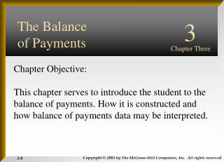
INTERNATIONAL FINANCIAL MANAGEMENT. Fourth Edition. EUN / RESNICK. 18. International Capital Budgeting. Chapter Eighteen. Chapter Objective: This chapter discusses the methodology that a multinational firm can use to analyze the investment of capital in a foreign country. INTERNATIONAL

E N D
INTERNATIONAL FINANCIAL MANAGEMENT Fourth Edition EUN / RESNICK
18 International Capital Budgeting Chapter Eighteen Chapter Objective: This chapter discusses the methodology that a multinational firm can use to analyze the investment of capital in a foreign country. INTERNATIONAL FINANCIAL MANAGEMENT Fourth Edition EUN / RESNICK
Chapter Outline • Review of Domestic Capital Budgeting • The Adjusted Present Value Model • Capital Budgeting from the Parent Firm’s Perspective • Risk Adjustment in the Capital Budgeting Process • Sensitivity Analysis • Real Options
Review of Domestic Capital Budgeting 1.Identify the SIZE and TIMING of all relevant cash flows on a time line. 2. Identify the RISKINESS of the cash flows to determine the appropriate discount rate. 3. Find NPV by discounting the cash flows at the appropriate discount rate. 4. Compare the value of competing cash flow streams at the same point in time.
Review of Domestic Capital Budgeting The basic net present value equation is Where: CFt = expected incremental after-tax cash flow in year t, TVT = expected after tax terminal value including return of net working capital, C0 = initial investment at inception, K = weighted average cost of capital. T = economic life of the project in years.
Review of Domestic Capital Budgeting The NPV rule is to accept a project if NPV 0 and to reject a project if NPV 0
Review of Domestic Capital Budgeting For our purposes it is necessary to expand the NPV equation. CFt = (Rt – OCt – Dt – It)(1 – t) + Dt + It(1 – t) Rt is incremental revenue OCt is incremental operating cash flow Dt is incremental depreciation It is incremental interest expense is the marginal tax rate
Alternative Formulations CFt CFt = (Rt – OCt – Dt – It)(1 – t) + Dt + It(1 – t) CFt = (NIt + Dt + It(1 – t) CFt = (Rt – OCt – Dt(1 – t) + Dt CFt = (NOIt)(1 – t) + Dt CFt = (Rt – OCt)(1 – t) + t Dt CFt = (OCFt)(1 – t) + t Dt
T CFt TVT S NPV = + – C0 (1 + K)t (1 + K)T t = 1 T (OCFt)(1 – t) + t Dt TVT S NPV = + – C0 (1 + K)t (1 + K)T t = 1 Review of Domestic Capital Budgeting We can use CFt = (OCFt)(1 – t) + t Dt to restate the NPV equation as:
T (OCFt)(1 – t) T t Dt TVT S S NPV = + + – C0 (1 + K)t (1 + K)t (1 + K)T t = 1 t = 1 T (OCFt)(1 – t) t Dt t It TVT S APV = + + + – C0 (1 + Ku)t (1+i)t (1+i)t (1+Ku)T t = 1 The Adjusted Present Value Model Can be converted to adjusted present value (APV) By appealing to Modigliani and Miller’s results.
T (OCFt)(1 – t) t Dt t It TVT S APV = + + + – C0 (1 + Ku)t (1+i)t (1+i)t (1+Ku)T t = 1 The Adjusted Present Value Model The APV model is a value additivity approach to capital budgeting. Each cash flow that is a source of value to the firm is considered individually. Note that with the APV model, each cash flow is discounted at a rate that is appropriate to the riskiness of the cash flow.
-$1,000 $125 $250 $375 $500 0 1 2 3 4 Domestic APV Example Consider this project, the timing and size of the incremental after-tax cash flows for an all-equity firm are: The unlevered cost of equity is r0 = 10%: CF0 = –$1000 The project would be rejected by an all-equity firm: CF1 = $125 CF2 = $250 I = 10 CF3 = $500 NPV = –$56.50
Domestic APV Example (continued) • Now, imagine that the firm finances the project with $600 of debt at r = 8%. • The tax rate is 40%, so they have an interest tax shield worth t×I = .40×$600×.08 = $19.20 each year.
T (OCFt)(1 – t) t Dt t It TVT S $125 $250 $375 $500 APV = + + + – C0 + + + (1 + Ku)t (1+i)t (1+i)t (1+Ku)T 1.10 (1.10)2 (1.10)3 (1.10)4 t = 1 $19.20 $19.20 $19.20 $19.20 + + + + 1.08 (1.08)2 (1.08)3 (1.08)4 -$1,000 $125 $250 $375 $500 0 1 2 3 4 The APV of the project under leverage is: APV = – $1,000 APV = $7.09 The firm should accept the project if it finances with debt.
T (OCFt)(1 – t) t Dt t It TVT S APV = + + + – C0 (1 + Ku)t (1+i)t (1+i)t (1+Ku)T t = 1 Capital Budgeting from the Parent Firm’s Perspective • The APV model is useful for a domestic firm analyzing a domestic capital expenditure or for a foreign subsidiary of a MNC analyzing a proposed capital expenditure from the subsidiary’s viewpoint. • The APV model is NOT useful for a MNC in analyzing a foreign capital expenditure from the parent firm’s perspective.
Capital Budgeting from the Parent Firm’s Perspective • Donald Lessard developed an APV model for a MNC analyzing a foreign capital expenditure. The model recognizes many of the particulars peculiar to foreign direct investment.
T T T StOCFt(1 – t) St St St St t Dt t It S S S APV = + + (1 + Kud)t (1+id)t (1+id)t t = 1 t = 1 t = 1 TVT T LPt S + – S0C0 + S0RF0 + S0CL0 + (1+Kud)T (1+id)t t = 1
T T T StOCFt(1 – t) St St St St t Dt t It S S S APV = + + (1 + Kud)t (1+id)t (1+id)t t = 1 t = 1 t = 1 TVT T LPt S + – S0C0 + S0RF0 + S0CL0 + (1+Kud)T (1+id)t t = 1 Capital Budgeting from the Parent Firm’s Perspective The operating cash flows must be translated back into the parent firm’s currency at the spot rate expected to prevail in each period. The operating cash flows must be discounted at the unlevered domestic rate
T T T StOCFt(1 – t) St St St St t Dt t It S S S APV = + + (1 + Kud)t (1+id)t (1+id)t t = 1 t = 1 t = 1 TVT T LPt S + – S0C0 + S0RF0 + S0CL0 + (1+Kud)T (1+id)t t = 1 Capital Budgeting from the Parent Firm’s Perspective OCFt represents only the portion of operating cash flows available for remittance that can be legally remitted to the parent firm. The marginal corporate tax rate, , is the larger of the parent’s or foreign subsidiary’s.
T T T StOCFt(1 – t) St St St St t Dt t It S S S APV = + + (1 + Kud)t (1+id)t (1+id)t t = 1 t = 1 t = 1 TVT T LPt S + – S0C0 + S0RF0 + S0CL0 + (1+Kud)T (1+id)t t = 1 Capital Budgeting from the Parent Firm’s Perspective S0RF0 represents the value of accumulated restricted funds (in the amount of RF0) that are freed up by the project. Denotes the present value (in the parent’s currency) of any concessionary loans,CL0, and loan payments, LPt , discounted at id .
Capital Budgeting from the Parent Firm’s Perspective One recipe for international decision makers: 1. Estimate future cash flows in foreign currency. 2. Convert to the home currency at the predicted exchange rate. Use PPP, IRP et cetera for the predictions. 3. Calculate NPV using the home currency cost of capital.
Capital Budgeting from the Parent Firm’s Perspective: Example • A U.S.-based MNC is considering a European opportunity. • It’s a simple example • There is no incremental debt • There is no incremental depreciation • There are no concessionary loans • There are no restricted funds
T T T StOCFt(1 – t) St St St St t Dt t It S S S APV = + + (1 + Kud)t (1+id)t (1+id)t t = 1 t = 1 t = 1 TVT T LPt S + – S0C0 + S0RF0 + S0CL0 + (1+Kud)T (1+id)t t = 1 T StOCFt(1 – t) S APV = –S0C0 (1 + Kud)t t = 1 Capital Budgeting from the Parent Firm’s Perspective: Example • We can use a simplified APV:
–€600 €200 €500 €300 0 1 3 2 Capital Budgeting from the Parent Firm’s Perspective: Example A U.S. MNC is considering a European opportunity. The size and timing of the after-tax cash flows are: The inflation rate in the euro zone is € = 3%, the inflation rate in dollars is p$ = 6%, and the business risk of the investment would lead an unlevered U.S. based firm to demand a return of Kud = i$ = 15%.
–€600 €200 €500 €300 0 1 3 2 $1.25 The current exchange rate is S0($/€)= € Capital Budgeting from the Parent Firm’s Perspective: Example Is this a good investment from the perspective of the U.S. shareholders? To address that question, let’s convert all of the cash flows to dollars and then find the NPV at i$ = 15%.
–€600 €200 €500 €300 0 1 3 2 $1.25 $1.25 S0($/€)= CF0 = (€600)× S0($/€) =(€600)× = $750 € € Capital Budgeting from the Parent Firm’s Perspective: Example –$750 Finding the dollar value of the initial cash flow is easy; convert at the spot rate:
–€600 €200 €500 €300 0 1 3 2 The exchange rate expected to prevail in the first year, S1($/€), can be found with PPP: 1 + $ S0($/€) S1($/€) = 1.06 $1.25 1 + € = 1.03 € CF1 = €200 × S1($/€) = €200 × $1.2864/€ = $257.28 Capital Budgeting from the Parent Firm’s Perspective: Example –$750 $257.28 = $1.2864/€
–€600 €200 €500 €300 0 1 3 2 1.06 1.06 $1.25 CF2 €500 = 1.03 1.03 € Capital Budgeting from the Parent Firm’s Perspective: Example –$750 $257.28 $661.94 = $661.94
–€600 €200 €500 €300 0 1 3 2 1.06 1.06 1.06 $1.25 CF3 €300 = $408.73 = 1.03 1.03 1.03 € Capital Budgeting from the Parent Firm’s Perspective: Example –$750 $257.28 $661.94 $408.73
–$750 $257.28 $661.94 $408.73 0 1 3 2 Capital Budgeting from the Parent Firm’s Perspective: Example Find the NPV using the cash flow menu of your financial calculator and and interest rate i$ = 15%: CF0 = –$750 CF1 = $257.28 CF2 = $661.94 I = 15 CF3 = $408.73 NPV = $242.99
–$750 $257.28 $661.94 $408.73 0 1 3 2 Capital Budgeting from the Parent Firm’s Perspective: Example Without a financial calculator, the NPV can be found as: $257.28 $661.94 $408.73 = $242.99 + + NPV = –$750 + 1.15 (1.15)2 (1.15)3
Capital Budgeting from the Parent Firm’s Perspective: Alternative Another recipe for international decision makers: 1. Estimate future cash flows in foreign currency. 2. Estimate the foreign currency discount rate. 3. Calculate the foreign currency NPV using the foreign cost of capital. 4. Translate the foreign currency NPV into dollars using the spot exchange rate
$1.25 The current exchange rate is S0($/€)= € – €600 €200 €500 €300 0 1 3 2 Foreign Currency Cost of Capital Method Let’s find i€ and use that on the euro cash flows to find the NPV in euros. Then translate the NPV into dollars at the spot rate. € = 3% i$ = 15% p$ = 6%
Foreign Currency Cost of Capital Method • Before we find i€ let’s use our intuition. • Since the euro-zone inflation rate is 3% lower than the dollar inflation rate, our euro denominated discount rate should be lower than our dollar denominated discount rate.
real rate inflation rate nominal rate (1 + i$) 1.15 (1 + e) = e = – 1 = 0.0849 (1 + $) 1.06 Finding the Foreign Currency Cost of Capital: i€ Recall that the Fisher Effect holds that (1 + e) × (1 + $) = (1 + i$) So for example the real rate in the U.S. must be 8.49%
(1 + i$) (1 + i€) (1 + i$) (1 + i€) = (1 + e$) = (1 + e€) = (1 + $) (1 + €) (1 + $) (1 + €) Finding the Foreign Currency Cost of Capital: i€ If Fisher Effect holds here and abroad then and If the real rates are the same in dollars and euros (e€ = e$) we have a very useful parity condition:
(1 + i$) (1 + i€) (1.15) × (1.03) = – 1 i€ = (1.06) (1 + $) (1 + €) (1 + i$) × (1 + €) (1 + i€) = (1 + $) Finding the Foreign Currency Cost of Capital: i€ If we have any three of these variables, we can find the fourth: In our example, we want to find i€ i€ = 0.1175
– €600 €200 €500 €300 0 1 3 2 $1.25 = $242.99 €194.39 × € International Capital Budgeting: Example Find the NPV using the cash flow menu and i€ = 11.75%: CF0 = –€600 I = 11.75 CF1 = €200 NPV = €194.39 CF2 = €500 CF3 = €300
– €600 €200 €500 €300 0 1 3 2 €200 €500 €300 = €194.39 + + NPV = –€600 + 1.1175 (1.1175)2 (1.1175)3 $1.25 = $242.99 €194.39 × € Capital Budgeting from the Parent Firm’s Perspective: Example Without a financial calculator, the NPV can be found as:
International Capital Budgeting • You have two equally valid approaches: • Change the foreign cash flows into dollars at the exchange rates expected to prevail. Find the $NPV using the dollar cost of capital. • Find the foreign currency NPV using the foreign currency cost of capital. Translate that into dollars at the spot exchange rate. • If you watch your rounding, you will get exactly the same answer either way. • Which method you prefer is your choice.
T T T StOCFt(1 – t) St St St St t Dt t It S S S APV = + + (1 + Kud)t (1+id)t (1+id)t t = 1 t = 1 t = 1 TVT T LPt S S0 S0 S0 S0 + – S0C0 + S0RF0 + S0CL0 + (1+Kud)T (1+id)t t = 1 f f f f f S0 Back to the full APV • Using the intuition just developed, we can modify Lessard’s APV model as shown above, if we find it convenient.
Risk Adjustment in the Capital Budgeting Process • Clearly risk and return are correlated. • Political risk may exist along side of business risk, necessitating an adjustment in the discount rate.
Sensitivity Analysis • In the APV model, each cash flow has a probability distribution associated with it. • Hence, the realized value may be different from what was expected. • In sensitivity analysis, different estimates are used for expected inflation rates, cost and pricing estimates, and other inputs for the APV to give the manager a more complete picture of the planned capital investment.
Real Options • The application of options pricing theory to the evaluation of investment options in real projects is known as real options. • A timing option is an option on when to make the investment. • A growth option is an option to increase the scale of the investment. • A suspension option is an option to temporarily cease production. • An abandonment option is an option to quit the investment early.
–£1,000 £1,150 0 1 €2.00 The current exchange rate is S0(€|£)= £ Value of the Option to Delay: Example A French firm is considering a one-year investment in the United Kingdom with a pound-denominated rate of return of 15%. The firm’s local cost of capital is i€ = 10% The cash flows are
Value of the Option to Delay: Example • Suppose that the bank of England is considering either tightening or loosening its monetary policy. • It is widely believed that in one year there are only two possibilities: • S1(€|£) = €2.20 per £ • S1(€|£) = €1.80 per £ • Following revaluation, the exchange rate is expected to remain steady for at least another year.
If S1(€|£) = €1.80 per £ the project will have turned out to be a loser for the French firm: If S1(€|£) = €2.20 per £ the project will have turned out to be a winner for the French firm: –€2,000 €2,070 –€2,000 €2,530 0 1 0 1 Option to Delay: Example IRR = 3.50% IRR = 26.50%
Option to Delay: Example • An important thing to notice is that there is an important source of risk (exchange rate risk) that isn’t incorporated into the French firm’s local cost of capital of i€ = 10%. • That’s why there are no NPV estimates on the last slide. • Even with that, we can see that taking the project on today entails a “win big—lose big” gamble on exchange rates. • Analogous to buying an at-the-money call option on British pounds with a maturity of one year.
Option to Delay: Example • The remaining slides assume a knowledge of the material contained in chapter 7. • Especially the notion of a replicating portfolio. • But also basic things like a call options gives the holder the right to buy a specific asset at a specific price for a specific amount of time.
British Investment Call Option Replicating Portfolio S1(€|£) = Bond + = €2.20/£ €2,530 = €2,070 + €460 = €2,530 €1.80/£ €2,070 = €2,070 + €0 = €2,070 Option to Delay: Example • The payoff in one year of portfolio consisting of an at-the-money call option written on £2,300 plus a risk-free bond with a future value of €2,070 equals the payoff of the British investment: