Aggregate Demand II: Effects of Shocks, Fiscal Policy, and Monetary Policy
Learn how to analyze the effects of shocks, fiscal policy, and monetary policy using the IS-LM model, and derive the aggregate demand curve. Explore theories about the Great Depression.

Aggregate Demand II: Effects of Shocks, Fiscal Policy, and Monetary Policy
E N D
Presentation Transcript
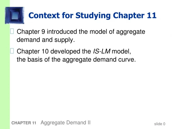
Context for Studying Chapter 11 • Chapter 9 introduced the model of aggregate demand and supply. • Chapter 10 developed the IS-LM model, the basis of the aggregate demand curve. CHAPTER 11 Aggregate Demand II
In Chapter 11, you will learn… • how to use the IS-LM model to analyze the effects of shocks, fiscal policy, and monetary policy • how to derive the aggregate demand curve from the IS-LM model • several theories about what caused the Great Depression CHAPTER 11 Aggregate Demand II
LM r IS Y Equilibrium in the IS-LMmodel The IScurve represents equilibrium in the goods market. r1 The LMcurve represents money market equilibrium. Y1 The intersection determines the unique combination of Y and rthat satisfies equilibrium in both markets. CHAPTER 11 Aggregate Demand II
LM r r1 IS Y1 Y Policy analysis with the IS-LM model We can use the IS-LM model to analyze the effects of • fiscal policy: G and/or T • monetary policy: M CHAPTER 11 Aggregate Demand II
LM r r2 r1 IS2 IS1 Y1 Y2 Y 2. 1. 3. An increase in government purchases 1. IS curve shifts right causing output & income to rise. 2. This raises money demand, causing the interest rate to rise… 3. …which reduces investment, so the final increase in Y CHAPTER 11 Aggregate Demand II
LM r r2 1. 2. r1 1. IS2 IS1 Y1 Y2 Y 2. 2. A tax cut Consumers save (1MPC) of the tax cut, so the initial boost in spending is smaller for T than for an equal G… and the IS curve shifts by …so the effects on rand Y are smaller for T than for an equal G. CHAPTER 11 Aggregate Demand II
LM1 r LM2 r1 r2 IS Y2 Y1 Y Monetary policy: An increase in M 1. M > 0 shifts the LM curve down(or to the right) 2. …causing the interest rate to fall 3. …which increases investment, causing output & income to rise. CHAPTER 11 Aggregate Demand II
Interaction between monetary & fiscal policy • Model: Monetary & fiscal policy variables (M, G, and T) are exogenous. • Real world: Monetary policymakers may adjust Min response to changes in fiscal policy, or vice versa. • Such interaction may alter the impact of the original policy change. CHAPTER 11 Aggregate Demand II
The B of C’s response to G > 0 • Suppose Parliament increases G. • Possible B of C responses: 1.hold M constant 2.hold r constant 3.hold Y constant • In each case, the effects of the Gare different: CHAPTER 11 Aggregate Demand II
LM1 r r2 r1 IS2 IS1 Y1 Y2 Y Response 1: Hold M constant If govt raises G, the IS curve shifts right. If B of C holds M constant, then LM curve doesn’t shift. Results: CHAPTER 11 Aggregate Demand II
LM1 r LM2 IS2 IS1 Y3 Y1 Y2 Y Response 2: Hold r constant If Congress raises G, the IScurve shifts right. To keep r constant, B of C increases Mto shift LM curve right. r2 r1 Results: CHAPTER 11 Aggregate Demand II
LM2 LM1 r r3 r1 IS2 IS1 Y1 Y2 Y Response 3: Hold Y constant If govt raises G, the IScurve shifts right. To keep Y constant, B of C reduces Mto shift LM curve left. r2 Results: CHAPTER 11 Aggregate Demand II
Estimates of fiscal policy multipliers from the DRI macroeconometric model Estimated value of Y/G Estimated value of Y/T Assumption about monetary policy B of C holds money supply constant 0.60 0.26 B of C holds nominal interest rate constant 1.93 1.19 CHAPTER 11 Aggregate Demand II
Shocks in the IS-LM model IS shocks: exogenous changes in the demand for goods & services. Examples: • stock market boom or crash change in households’ wealth C • change in business or consumer confidence or expectations I and/or C CHAPTER 11 Aggregate Demand II
Shocks in the IS-LM model LM shocks: exogenous changes in the demand for money. Examples: • a wave of credit card fraud increases demand for money. • more ATMs or the Internet reduce money demand. CHAPTER 11 Aggregate Demand II
EXERCISE:Analyze shocks with the IS-LM model Use the IS-LM model to analyze the effects of 1.a boom in the stock market that makes consumers wealthier. 2.after a wave of credit card fraud, consumers using cash more frequently in transactions. For each shock, a.use the IS-LM diagram to show the effects of the shock on Y and r. b.determine what happens to C, I, and the unemployment rate. CHAPTER 11 Aggregate Demand II
IS-LM and aggregate demand • So far, we’ve been using the IS-LMmodel to analyze the short run, when the price level is assumed fixed. • However, a change in P would shift LM and therefore affect Y. • The aggregate demand curve(introduced in Chap. 9) captures this relationship between P and Y. CHAPTER 11 Aggregate Demand II
r P LM(P2) LM(P1) r2 r1 IS Y Y P2 P1 Deriving the AD curve Intuition for slope of AD curve: P (M/P) LM shifts left r I Y Y1 Y2 AD Y2 Y1 CHAPTER 11 Aggregate Demand II
r P LM(M1/P1) LM(M2/P1) r1 r2 IS Y Y Y2 Y1 P1 AD2 AD1 Y1 Y2 Monetary policy and the AD curve The B of C can increase aggregate demand: M LM shifts right r I Y at each value of P CHAPTER 11 Aggregate Demand II
r P LM r2 r1 IS2 IS1 Y Y Y2 Y1 P1 AD2 AD1 Y1 Y2 Fiscal policy and the AD curve Expansionary fiscal policy (G and/or T) increases agg. demand: T C IS shifts right Y at each value of P CHAPTER 11 Aggregate Demand II
IS-LM and AD-AS in the short run & long run Recall from Chapter 9: The force that moves the economy from the short run to the long run is the gradual adjustment of prices. In the short-run equilibrium, if then over time, the price level will rise fall remain constant CHAPTER 11 Aggregate Demand II
LRAS r P LM(P1) IS1 IS2 Y Y LRAS SRAS1 P1 AD1 AD2 The SR and LR effects of an IS shock A negative IS shock shifts IS and AD left, causing Y to fall. CHAPTER 11 Aggregate Demand II
LRAS r P LM(P1) IS2 Y Y SRAS1 P1 AD2 The SR and LR effects of an IS shock In the new short-run equilibrium, IS1 LRAS AD1 CHAPTER 11 Aggregate Demand II
LRAS r P LM(P1) IS2 Y Y SRAS1 P1 AD2 The SR and LR effects of an IS shock In the new short-run equilibrium, IS1 Over time, P gradually falls, which causes • SRAS to move down. • M/P to increase, which causes LMto move down. LRAS AD1 CHAPTER 11 Aggregate Demand II
LRAS r P LM(P2) IS2 Y Y SRAS2 P2 AD2 The SR and LR effects of an IS shock LM(P1) IS1 Over time, P gradually falls, which causes • SRAS to move down. • M/P to increase, which causes LMto move down. LRAS SRAS1 P1 AD1 CHAPTER 11 Aggregate Demand II
LRAS P r LM(P2) IS2 Y Y SRAS2 P2 AD2 The SR and LR effects of an IS shock LM(P1) This process continues until economy reaches a long-run equilibrium with IS1 LRAS SRAS1 P1 AD1 CHAPTER 11 Aggregate Demand II