Download
1 / 22
220 likes | 297 Vues
Explore the Higgs mechanism in quantum field theory, explaining how it generates mass, introduces gauge fields, and alters theories of particle physics. Delve into the mathematical foundations and implications for fundamental particles.

E N D
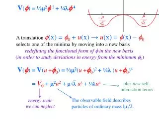
√λ √λ V(f) = ½2 + ¼4 - A translation f(x) = f0 + u(x)→ u(x) ≡ f(x) – f0 selects one of the minima by moving into a new basis redefining the functional form of f in the new basis (in order to study deviations in energy from the minimum f0) V(f) = V(u+f0) = ½(u+f0)2 + ¼ (u+f0)4 = V0+u2+ √ u3+ ¼u4 plus new self- interaction terms The observable field describes particles of ordinary mass |m|/2. energy scale we can neglect
U U 1 some calculus of variations Letting = * = 0 U 2 = 0 Extrema occur not only for but also for But since = * This must mean-2 > 0 2 < 0 > 0 and I guess we’ve sort of been assuming was a mass term!
2 defines a circle of radius || / in the 2vs1 plane Furthermore, from 1 U 1 not x-y “space” we note 2U 12 which at = 0gives just2 < 0 making = 0the location of a local MAXIMUM!
Lowest energy states exist in this circular valley/rut of radius v = 2 1 This clearly shows the U(1)SO(2) symmetry of the Lagrangian But only one final state can be “chosen” Because of the rotational symmetry all are equivalent We can chose the one that will simplify our expressions (and make it easier to identify the meaningful terms) shift to the selected ground state expanding the field about the ground state:1(x)=+(x)
Scalar (spin=0) particle Lagrangian L=½11 + ½22 ½12+22 ¼12+22 with these substitutions: v = L=½ + ½ ½2+2v+v2+2 ¼2+2v+v2+2 becomes L=½ + ½ ½2+ 2 v ½v2 ¼2+2 ¼22+22v+v2 ¼2v+v2
L=½ + ½ ½(2v)2 v2+2¼2+2 + ¼v4 ½ ½(2v)2 Explicitly expressed in real quantities and v this is now an ordinary mass term! “appears” as a scalar (spin=0) particle with a mass ½ “appears” as a massless scalar There is NO mass term!
Of course we want even this Lagrangian to be invariant to LOCAL GAUGE TRANSFORMATIONS D=+igG Let’s not worry about the higher order symmetries…yet… free field for the gauge particle introduced Recall: F=G-G * 12 + i22 again we define: 1 + i2
so, also as before: with Note: v =0 Exactly the same potentialU as before!
L= [+ v22] + [ ] + [ FF+ GG] -gvG 1 2 g2v2 2 1 2 -1 4 +{ g2 2 gG[-] + [2+2v+2]GG 2 1 2 + [2v3+v4+2v2 - (4+43v+62v2+4v3+4v2 + 222+2v22+v4 + 4 ) ]} L= [+ v22] + [ ] + [ FF+ GG] -gvG 1 2 g2v2 2 1 2 -1 4 +{ g2 2 gG[-] + [2+2v+2]GG 4 2 1 2 - [4v(3+2) + [ v4] + [4+222+ 4] and many interactions between and which includes a numerical constant v4 4
The constants , v give the coupling strengths of each
which we can interpret as: a whole bunch of 3-4 legged vertex couplings massless scalar free Gauge field with mass=gv scalar field with L = -gvG + + + But no MASSLESS scalar particle has ever been observed is a ~massless spin-½ particle is a massless spin-1particle spinless,have plenty of mass! plus - gvG seems to describe G • Is this an interaction? • A confused mass term? • G not independent? ( some QM oscillation between mixed states?) Higgs suggested:have not correctly identified the PHYSICALLY OBSERVABLE fundamental particles!
RememberLisU(1)invariant - rotationally invariant in , (1, 2) space – i.e. it can be equivalently expressed under any gauge transformation in the complex plane Note: or /=(cos + isin )(1 + i2) =(1cos-2sin ) + i(1sin+ 2cos) With no loss of generality we are free to pick the gaugea , for example, picking: /2 0 and/ becomes real!
ring of possible ground states equivalent to rotating the system by angle - 2 1 (x) (x) = 0
£ With real, the field vanishes and our Lagrangian reduces to introducing a MASSIVE Higgs scalar field, , and “getting” a massive vector gauge field G Notice, with the field gone, all those extra , , and interaction terms have vanished Can we employ this same technique to explain massive Z and W vector bosons?
Now apply these techniques: introducing scalar Higgs fields • with a self-interaction term and then expanding fields about the • ground state of the broken symmetry • to theSUL(2)×U(1)YLagrangianin such a way as to • endow W,Zs with mass but leave s massless. These two separate cases will follow naturally by assuming the Higgs field is aweak iso-doublet(with a charged and uncharged state) withQ = I3+Yw /2and I3 = ±½ Higgs= + 0 for Q=0Yw = 1 Q=1Yw = 1 couple to EW UY(1) fields: B
+ 0 £ £ Higgs= withQ=I3+Yw /2and I3 = ±½ Yw = 1 Consider just the scalar Higgs-relevant terms † † † with Higgs not a single complex function now, but a vector(an isodoublet) Once again with each field complex we write + = 1 + i2 0= 3 + i4 † 12 + 22 + 32 + 42 † † † Higgs † † † †
L † † † Higgs † † † † just like before: U=½m2† + ¹/4 († )2 -2m2 12 + 22 + 32 + 42= Notice how 12, 22 … 42appear interchangeably in the Lagrangian invariance to SO(4) rotations Just like with SO(3) where successive rotations can be performed to align a vector with any chosen axis,we can rotate within this 1-2-3-4 space to a Lagrangian expressed in terms of a SINGLE PHYSICAL FIELD
Were we to continue without rotating the Lagrangian to its simplest terms we’d find EXTRANEOUS unphysical fields with the kind of bizarre interactions once again suggestion non-contributing “ghost particles” in our expressions. + 0 Higgs= So let’s pick ONE field to remain NON-ZERO. 1or2 3or4 because of the SO(4) symmetry…all are equivalent/identical might as well make real! v+H(x) 0 0 v+H(x) Can either choose or But we lose our freedom to choose randomly. We have no choice. Each represents a different theory with different physics!
Let’s look at the vacuum expectation values of each proposed state. v+H(x) 0 0 v+H(x) or Aren’t these just orthogonal? Shouldn’t these just be ZERO? Yes, of course…for unbroken symmetric ground states. If non-zero would imply the “empty” vacuum state “OVERLPS with” or contains (quantum mechanically decomposes into) some of + or 0. But that’s what happens in spontaneous symmetry breaking: the vacuum is redefined “picking up” energy from the field which defines the minimum energy of the system.
a non-zero v.e.v.! = v 0 1 This would be disastrous for the choice + = v + H(x) since0|+ = vimplies the vacuum is not chargeless! But 0| 0 = v is an acceptable choice. If the Higgs mechanism is at work in our world, this must be nature’s choice.
Let’s recap: We’ve worked through 2 MATHEMATICAL MECHANISMS for manipulating Lagrangains Introducing SELF-INTERACTION terms (generalized “mass” terms) showed that a specific GROUND STATE of a system need NOT display the full available symmetry of the Lagrangian Effectively changing variables by expanding the field about the GROUND STATE (from which we get the physically meaningful ENERGY values, anyway) showed • The scalar field ends up with a mass term; a 2nd (extraneous) • apparently massless field (ghost particle) can be gauged away. • Any GAUGE FIELD coupling to this scalar (introduced by • local invariance) acquires a mass as well!
We then applied these techniques by introducing the scalar Higgs fields through a weak iso-doublet (with a charged and uncharged state) + 0 0 v+H(x) Higgs= = which, because of the explicit SO(4) symmetry, the proper gauge selection can rotate us within the1,2,3,4space, reducing this to a single observable real field which we we expand about the vacuum expectation value v.