Download
1 / 15
150 likes | 312 Vues
Underwater Radiance Field with Dynamic Surface Waves. George W. Kattawar and Yu You Department of Physics Texas A&M University. Outline. Methods A “realistic” surface wave model Underwater radiance field with dynamic surface waves

E N D
Underwater Radiance Field with Dynamic Surface Waves George W. Kattawar and Yu You Department of Physics Texas A&M University
Outline • Methods • A “realistic” surface wave model • Underwater radiance field with dynamic surface waves • Image of an object above the surface with dynamic surface waves
Methods - the Matrix Operator (MO) Method Z Atmosphere, Slow Changing Part Ocean Wave, Fast Changing part Detector Ocean, Slow Changing Part Lambertian Ocean Bottom X
Methods - Previous Work • The MO code validated for a plane-parallel system • MO simulations of system with 1-D and 2-D sinusoidal surface waves • Needs measurements of surface wave slopes for further simulation
A “Realistic” Surface Wave Model • Modeling of gravity waves and swells using the power spectral density (PSD) approach. Schwenger and Repasi, Proc. of SPIE, 5075, 72 (2003) : Phases are generated with a Gaussian distribution
A “Realistic” Surface Wave Model Simulated Gravity Waves Wind speed: W = 5 m/s Wind speed: W = 10 m/s Area: 21 m x 21 m
A “Realistic” Surface Wave Model Comparison with Cox-Munk Results Lines - Direct Monte Carlo results using the Cox-Munk model Symbols - MO results with “realistic” surface waves (averaged over 225 grids) Atmosphere: Rayleigh = 0.25, = 0.5 Ocean: H-G, g = 0.95 = 10, = 0.5 Bottom: Lambertian = 0.5 Detector: = 0.001 SZA = 0 degree Atmosphere & ocean: 15 x 15 grids Interface: 255 x 255 grids
A “Realistic” Surface Wave Model Simulated Gravity Waves and Swells Wind speed: W = 10 m/s
Underwater radiance field with dynamic surface waves Radiance at Various Depths det 0.001 1 2 5
Underwater radiance field with dynamic surface waves Q Component at Various Depths det 0.001 1 2 5
Underwater radiance field with dynamic surface waves U Component at Various Depths det 0.001 1 2 5
Image of an object with dynamic surface waves Image of a Disk - Flat surface det = 1 A disk just above the ocean surface r = 4.5 m
Image of an object with dynamic surface waves A Dynamic Ocean Surface det = 1 r = 4.5 m det = 2
Image of an object with dynamic surface waves A Smaller Disk - Flat Surface Radius of the disk: (inner circle) det = 5 Foot print of the Snell’s cone: 5.62 m (outer circle)
Image of an object with dynamic surface waves A Smaller Disk - Dynamic Ocean Radius of the disk: (inner circle) det = 5 Foot print of the Snell’s cone: 5.62 m (outer circle)