Statistical Thermodynamics: Understanding Partition Function Calculation
Learn about Boltzmann statistics, partition functions, and their impact on thermodynamic properties in gases. Explore advantages and limitations of microcosmic and macrocosmic properties in thermodynamics.

Statistical Thermodynamics: Understanding Partition Function Calculation
E N D
Presentation Transcript
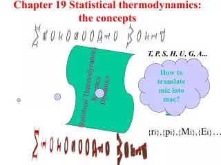
Content 3.1 Introduction 3.2 Boltzmann statistics 3.3 Partition function 3.4 Calculation of partition function 3.5 Contribution of Q to thermo_function 3.6 Calculation of ideal gas function
3.1 Introduction 3.1.1 Method and target According to the Stat. Unit mechanic properties (such as rate, momentum, vibration) are related with the system microcosmic and macrocosmic properties, work out the thermo-dynamics properties through the Stat. average. According to some basic suppositions of the substance structure,
and the spectrum data which get from the experiments, we can get some basic constant of the substance structure, such as the space between the nucleus, bond angle, vibration frequency and so on to work out the molecule partition function. And then according to the partition function we can work out the substance’s thermo-dynamics properties.
3.1.2 Advantage Related with the system microcosmic and macrocosmic properties, it is satisfied for some results we get from the simple molecule. No need to carry out the complicated low temperature measured heat experiment, then we can get the quite exact entropy.
3.1.3 Disadvantage The structure model must be supposed when calculating, certain approximate properties exist; for large complicated molecules and the agglomerated system, it still has some difficulties in calculating.
3.1.4 Localized system Particles can be distinguished from each other. For example, in the crystal, particles vibrate in the local crystal position, every position can be imagined to have different numbers to be distinguished, so the micro-cosmic state number of localized system is very large.
3.1.5 Non-localized system Basic particles can not be distinguished from each other. Such as, the gas molecule can not be distinguished from each other. When the particles are the same,its micro- cosmic state number is less than the localized system.
3.1.6 Assembly of independent particles The reciprocity of the particles is very faint, therefore it can be ignored, the total energy of the system is equal to the summation of every particles energy, that is:
3.1.7 Kinds of statistical system Maxwell-Boltzmann statistics usually called Boltzmann statistics Bose-Einstein statistics Fermi-Diracstatistics
3.2 Boltzmann Statistics Microcosmic state number of localized system Most probable distribution of localized system Degeneration Degeneration and Microcosmic state number Most probable distribution of non-localized system The other form of Boltzmann formula Entropy in Helmholz free energy expression
3.2.1 Microcosmic state number of localized system One macrocosmic system which is consisted by N independent particles which can be extinguished, it has many different partition forms in the quantitative level. Suppose one of the partition forms is: energy level ε1,ε2,· · · , εi one distributed form N1,N2,· · · ,Ni
3.2.1.2 The microcosmic state number of this partition is:
3.2.1.3 There are many forms of partition, the total microcosmic state number is: No matter what partition, it has to satisfy the following two conditions:
3.2.2 Most probable distribution of localized system The Ωi of every distribution is different but there is a maximal value Ωmax among them, in the macrocosmic system which has enough particles, the whole microcosmic number can approximately be replaced byΩmax, this is the most probable distribution.
3.2.2.1 The problem is how to find out a appropriate distribution Ni under two limit conditions to make Ω the max one, in mathematics, this is the question how to work it out under the conditional limit of formula (1). That is: ( work out the extreme, make
3.2.2.2 Firstly, outspread the factorial by the String formula, then use the methods of Lagrange multiply gene, the most probable distribution we get : The α and β in the formula is the non-fixed gene which are brought in by the methods of Lagrange multiply gene.
3.2.2.2 Most probable distribution of localized system Work it out by the mathematics methods: or So the most probable distribution formula is:
3.2.3 Degeneration Energy is quantitative, but probably several different quanta state exist in every energy level, the reflection on spectrum is that the spectrum line of certain energy level usually consisted by several very contiguous exact spectrum line . In the quanta mechanics,the probable micro- cosmic state number of energy level is called the degeneration of that energy level, we use gi to stand for it.
3.2.3.1 For example, the translation energy formula of the gas molecule is: The nx, ny and nz are the translation quantum numbers which separately in
3.2.3.2 so nx =1, ny =1 and nz=1, it only has one probable state, so gi=1, it is non-degeneration. the x, y and z axis,
3.2.3.3 At this moment, under the situation εi are the same, it has three different microcosmic states, so gi=0. When
3.2.4 Degeneration and Microcosmic state number Suppose one distribution of certain localized system which has N particles: Energy level ε1, ε2,· · · ,εi Every energy level degeneration g1,g2,· · · ,gi One distributed form N1,N2,· · · ,Ni
3.2.4.2 Choose N1 particles from N particles and then put them in the energy level ε1, there are CNN1 selective methods; But there are g1 different state in the ε1 energy level, every particle in energy level ε1 has g1 methods, so it has gN11methods; Therefore, put N1 particles in energy level ε1, it has gN11CNN1 microcosmic number. Analogy in turns, the microcosmic number of this distribution methods is:
3.2.4.4 Because there are many distribution forms, under the situation which U, V and N are definite, the total microcosmic state numbers are: The limit condition of sum still is:
3.2.4.5 Use the most probable distribution principle, ΣΩ1≈Ωmax , use the Stiring formula and Lagrange multiply gene method to work out condition limit, when the microcosmic state number is the maximal one, the distribution form N*i is:
3.2.4.6 Compare with the most probable distribution formula when we do not consider degeneration , it has an excessive item gi.
3.2.5 Most probable distribution of non-localized system Because particles can not be distinguished in the non-localized system, the microcosmic number which distribute in the energy level is less than the localized system, so amend the equal particle of the localized system microcosmic state number formula, that is the calculation formula divides N!
3.2.5 Most probable distribution of non-localized system Therefore, under the condition that U, V and N are the same, the total microcosmic state number of the non-localized system is:
3.2.5.2 Most probable distribution of non-localized system Use the most probable distribution principle, use the Stiring formula and Lagrang multiply gene method to work out the condition limit,when the micro-cosmic state number is the maximal one, the distribution form N*i (non-localized) is:
3.2.5.2 Most probable distribution of non-localized system It can be seen that the most probable distribution formula of the localized and non-localized system.
3.2.6 The other form of Boltzmann formula (1) Compare the particles of energy level i to j, use the most probable distribution formula to compare, expurgated the same items, then we can get:
3.2.6.2 The other form of Boltzmann formula (2) Degeneration is not considered in the classical mechanics, so the formula above is Suppose the lowest energy level is ε0, εi - ε0 =Δεi , the particles in ε0 energy level is N0, omit “*”, so the formula above can be written as:
3.2.6.2 The other form of Boltzmann formula This formula can be used conveniently, such as when we discuss the distribution of pressure in the gravity field, suppose the temperature is the same though altitude changes in the range from 0 to h, then we can get it.
3.2.7 Entropy in Helmholz free energy expression According to the Boltzmann formula which expose the essence of entropy (1) for localized system, non-degeneration
3.2.7.2 Entropy in Helmholz free energy expression Outspread of Stiring formula:
3.2.7.3 Entropy in Helmholz free energy expression
3.2.7.4 Entropy in Helmholz free energy expression (2) for localized system, degeneration is gi The deduce methods is similar with the previous one,among the results we get, the only excessive item than the result of (1) is item gi.
3.2.7.5 Entropy in Helmholz free energy expression (3) for the non-localized system Because the particles can not be distinguished, it need to equally amended, divide N! in the corresponding localized system formula, so:
3.3 Partition function 3.3.1 definition According to Boltzmann the most probable distribution formula (omit mark “.”) Cause the sum item of the denominator is:
3.3 Partition function q is called molecule partition function, or partition function, its unit is 1. The e-εi/kT in the sum item is called Boltzmann gene.The partition function q is the sum of every probable state Bolzmann gene of one particle in the system, so q is also called state summation.
3.3.1.2 Definition The comparison of any item in q; The comparison of any two items in q.
3.3.2 Separation of partition function The energy of one molecule is considered as the summation of the Translation energy of whole particles motion and the inner motionenergy of the molecule. The inner energy concludes the Translation energy (εr), Vibration energy (εv), electron energy (εe)and atom nucleus energy (εn), all of the energy can be considered to be independent.
3.3.2.2 Separation of partition function The total energy of molecule is equal to the summation of every energy Every different energy has corresponding degeneration, when the total energy is εi , the total degeneration is equal to the product of every energy degeneration, that is:
3.3.2.3 Separation of partition function According to the definition of partition function, put the expressions of εi and gi into it, then we can get:
3.3.2.3 Separation of partition function It can be proved in the mathematics, the product summation of several independent variables is equal to the separate product summation, so the formula above can be written as:
3.3.2.4 Separation of partition function qt, qr, qv, qe and qn are separately called Translation, Turn, Vibration, Electron, and atomic nucleus partition functions.
3.3.2.5 Separation of partition function Suppose the total particles is N (1) Helmholz free energy F
3.3.3 Relation between Q and thermodynamics function (2) entropy S Or we can get the following formula directly according to the entropy expression which was get before.