Solving Quality Control Problems Using Genetic Algorithms
This research, led by Douglas C. Montgomery and collaborators, explores the application of Genetic Algorithms (GAs) to solve complex quality control optimization problems. The study highlights the inspection problem faced by a medical device manufacturer, focusing on optimizing inspection parameters while adhering to budget constraints. By leveraging GAs, the team achieved significant cost savings, enhancing average outgoing quality compared to traditional methods. The innovative approaches demonstrated in this work showcase the potential of GAs to address multifaceted quality control challenges across various industries.

Solving Quality Control Problems Using Genetic Algorithms
E N D
Presentation Transcript
Solving Quality Control Problems Using Genetic Algorithms Douglas C. Montgomery Professor of Engineering and Statistics Arizona State University doug.montgomery@asu.edu
This is joint work with: • Alejandro Heredia-Langner, Pacific Northwest Labs (former PhD student, ASU) • W. Matthew Carlyle, Naval Postgraduate School (former IE faculty member, ASU) • Connie M. Borror, IE faculty member, ASU • George C. Runger, IE faculty member, ASU
Many problems in quality control involve complicated optimization problems • The inspection problem … Stage m Stage 1 Stage 2 nm, cm n1, c1 n2, c2 Carlyle, W. M., Montgomery, D. C., and Runger, G. C. (2000), “Optimization Problems and Methods in Quality Control and Improvement” (with discussion), Journal of Quality Technology, Vol. 32, No. 1, pp. 1-31.
In the inspection problem we wish to • Determine the parameters of the inspection scheme (the n’s and the c’s) • Optimize some important measure of effectiveness, such as maximize average outgoing quality at the final stage (m) • Not exceed a budget for inspection • Other criteria are also encountered in practice
The inspection problem was brought to our attention by a medical device manufacturer • FDA mandated inspections at each stage • m = 6 stages • Inspection is expensive, so is cost of inspection errors • Their solution was to “guess” at the n’s and c’s (simple but ugly) • Optimal solution involves dynamic programming (elegant but still ugly)
Genetic Algorithms • Initially created by the computer science community to study the behavior of simple, communal individuals under controlled conditions • Currently used as a tool to solve combinatorial optimization problems • Genetic Algorithms (GA) are loosely based on Darwin’s theory of evolution where a number of individuals compete for a limited amount of resources (survival of the fittest) • Mutation, mating and natural selection are implemented using individuals (or chromosomes) coded as strings of numbers (genes) • The fitness of these solutions is measured using an appropriate objective function
The GA methodology • A chromosome is a potential problem solution, a vector whose entries (or genes) represent the decision variables in the problem -0.4207 -1 0.0004 -0.7779 0.7786 0.4214 1 0.688783 Fitness value • Every solution or chromosome can be evaluated with respect to an objective function, resulting in a fitness value • Binary versus real encoding
How do GAs work? - Creating the new generation Parent population of many solutions Offspring created by recombination Pick two Combine
Effect of recombination • Original parent • Original parent
Some recombination mechanisms • Discrete - Two distinct chromosomes are selected at random and broken (also at random) in two or more places. The new individual is formed by adjoining pieces of alternate parents. • Generalized - Two chromosomes are chosen at random and the genes of the new individual formed as a convex combination of the parents (only for real-valued chromosomes) • Panmictic - Chromosomes are selected successively and each provides one entry for the new individual
Selection Offspring After recombination, rank the offspring chromosomes by fitness value and choose the best ones . . . . . . . . . . . . New Parent population
Some selection mechanisms • Proportional - Chromosomes are chosen using some biased probabilistic method where fitter individuals stand a better chance of being selected • Ranking - Offspring chromosomes are ranked according to fitness value and the new parent population formed choosing the best individuals sequentially • Extinctive - Some individuals are explicitly excluded from the selection process (this can be implemented with any of the above procedures)
+ Original parent Mutation Likely position of offspring A few of the individuals in the parent population are altered using normally distributed disturbances. This is called Gaussian mutation. Random uniform mutation replaces selected genes with others chosen from the available pool.
0 . 9 5 0 . 9 0 y t i l i b a r i s 0 . 8 5 e D 0 . 8 0 0 1 0 2 0 3 0 4 0 G e n e r a t i o n Effect of different types of mutation on fitness Gaussian Mutation Uniform Mutation No Mutation
Some results for the inspection problem • Use of the GA resulted in an annual savings of about $250K over the current “best-guess” solution • AOQ was approximately the same • Solved several other variations of the problem with different (multiple) objectives, including maximizing the probability of lot acceptance at each stage • Couldn’t do this with the DP approach Heredia-Langner, A., Montgomery, D. C., and Carlyle, W. M. (2002), “Solving a Multistage Partial Inspection Problem using Genetic Algorithms”, International Journal of Production Research, Vol. 40, No. 8, pp. 1923-1940.
GAs and Experimental Design • We use designed experiments to obtain information about how some independent variables affect the response (or responses) of interest • Our objective is usually to find a simple model for that relationship • If an adequate model is found, it can be employed for factor screening or to optimize the values of the responses • Good experimental designs use resources effectively and efficiently • There are many “standard” designs (factorials, fractional factorials, central composite, etc.)
What designs should be used? • If we have a “regular”experimental region +1 Concentration +1 Temperature -1 -1 -1 Pressure +1 • Then, most of the time, we know what kind of experiment (number and position of trials) we want to run
Why do we use “optimal” or computer-generated designs? • Useful whenever we cannot employ more traditional designs (full or fractional factorials...) due to: • Natural constraints in the design space (such as mixture experiments) • Unusual requirements for sample sizes or block sizes • The model under consideration is not standard • Cost, time, run order or other restrictions • In these cases we would still like to employ a set of experimental runs that are, in some sense, good
Some “Alphabetic” Design Optimality Criteria • Maximize the precision of estimation of the parameters in the proposed model (D) • Minimize the sum of the variances of the estimates of the model parameters (A) • Minimize the maximum variance of an estimated model parameter (E) • Minimize the average prediction variance of the model throughout the experimental region (V, Q or IV) • Cover the design region uniformly (S) • Minimize the maximum prediction variance (G) • Just about anything else that can yield a reasonable design (including a combination of the criteria above)
Some optimality criteria • D-optimality seeks to minimize the volume of the joint confidence region of the model parameters. It can be expressed as a determinant maximization problem • Q-optimality minimizes the average scaled prediction variance over the entire design region (the m identifies an experimental run in model form)
Methods for Constructing Alphabetically Optimal Designs • Exchange algorithms • Most widely used • Basis of commercial software packages • Branch and bound algorithms (Welch, 1982) • Simulated annealing (Haines, 1987) • Genetic algorithms (relatively recent) Hamada, M., Martz, H. F., Reese, C. J., and Wilson, A. G (2001), “Finding Near-Optimum Bayesian Experimental Designs Via Genetic algorithms”, The American Statistician, Vol. 55, pp. 175-181 Heredia-Langner, A., Carlyle, W. M., Montgomery, D. C., Borror, C. M., and. Runger, G. C. (2003), “Genetic Algorithms for the Construction of D-Optimal Designs”, to appear in the Journal of Quality Technology.
Example : A mixture problem with one processing variable • The objective is to find a G-optimal design (minimize the maximum prediction variance over the feasible region)
Results • Both the original method (B&B) and the GA are able to find the same design but… • The best design reported in the original reference was found after running the D-optimal algorithm multiple times and not by using the G-optimal algorithm • The G-optimal algorithm in the original reference was unable to find a good design 1/Fitness
Example: Model-Robust Efficient Designs Consider the problem of destructively sampling a radioactive rod so that its concentration of active material as a function of length can be modeled with a polynomial equation This problem originally appeared in Cook, R.D. and Nachtsheim, C. J. (1982). “Model-Robust, Linear-Optimal Designs.” Technometrics 24, pp. 49-54.
Creating Model-Robust Efficient Designs • Up to seven samples could be taken and analyzed • Models ranging from a simple linear to a sixth-degree polynomial were considered as equally likely candidates We are interested in modeling concentration as a function of position, but we don’t know which model is appropriate
1 0.95 0.9 0.85 0.8 0.75 0.7 1 2 3 4 5 6 Some results Cook and Nachtsheim GA Order of model The efficiencies of simpler models are always affected the most
Some Results • The solution method employed by the original researchers (based on an exchange method) can only handle one-variable designs • This isn’t a problem for the GA • The model-robust design problem is a very commonly-encountered version of the optimal design problem, and it’s notoriously ugly • The GA can provide very good solutions to some quite complex model-robust design problems Heredia-Langner, A., Montgomery, D. C., Carlyle, W. M., and Borror, C. M.(2002), “Model-Robust Optimal Designs: A Genetic Algorithm Approach”, in revision at the Journal of Quality Technology.
Conclusions • GAs can be used to construct a variety of efficient experimental designs • GAs work well for some of the most common design optimality criteria and even for some non-traditional ones • GAs are usually very effective for large, complex experimental design problems for which other methods may not work at all. This makes design efficiency comparisons difficult • GAs can be applied to many of the most common types of optimization problems encountered in statistical quality control and improvement