Component Labeling
Component Labeling. Scan the image left to right, top to bottom. If the pixel is 1, then If only one of its upper and left neighbors has a label, then copy the label. If both have the same label, then copy the label.

Component Labeling
E N D
Presentation Transcript
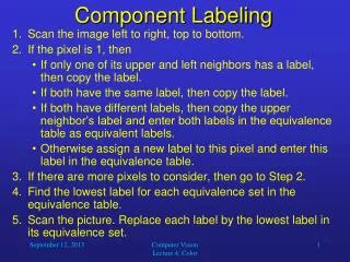
Component Labeling • Scan the image left to right, top to bottom. • If the pixel is 1, then • If only one of its upper and left neighbors has a label, then copy the label. • If both have the same label, then copy the label. • If both have different labels, then copy the upper neighbor’s label and enter both labels in the equivalence table as equivalent labels. • Otherwise assign a new label to this pixel and enter this label in the equivalence table. • If there are more pixels to consider, then go to Step 2. • Find the lowest label for each equivalence set in the equivalence table. • Scan the picture. Replace each label by the lowest label in its equivalence set. Computer Vision Lecture 4: Color
Size Filter • We can use component labeling to remove noise in binary images. • For example, when we want to perform optical character recognition (OCR), it often happens that there are small groups of 1-pixels outside the actual characters. • Since these are usually very small, isolated blobs, we can remove them by applying a size filter, that is, • labeling all components, • computing their size, and • for all components smaller than a threshold T, setting all of their pixels to 0. Computer Vision Lecture 4: Color
Size Filter • Here, for T = 10, the size filter perfectly removes all noise in the input image. Computer Vision Lecture 4: Color
Size Filter • However, if our threshold is too high, “accidents” may happen. Computer Vision Lecture 4: Color
Size Filter • In the case we had only “positive noise,” that is, there were some 1-pixels in places that should have contained 0-pixels, • Often, we also have “negative noise,” which means that we have 0-pixels in places that should contain 1-pixels. • To remove negative noise, we could define a “hole size filter” that removes all holes that are smaller than a certain threshold. • A common, efficient method of removing both kinds of noise is to apply sequences of expanding and shrinking. Computer Vision Lecture 4: Color
Expanding and Shrinking • As we have just seen, using a size filter is one method for preprocessing images for subsequent character recognition. • Another common way of achieving this is called expanding and shrinking. • Expanding operation: For all pixels in the image, change a pixel from 0 to 1 if any neighbors of the pixel are 1. • Shrinking operation: For all pixels in the image, change a pixel from 1 to 0 if any neighbors of the pixel are 0. Computer Vision Lecture 4: Color
Expanding and Shrinking Here, the original image (left) is expanded (center) or shrunken (right). Shrinking can actually be considered as expanding the background. Computer Vision Lecture 4: Color
Expanding and Shrinking • Expanding followed by shrinking can be used for filling undesirable holes. • Shrinking followed by expanding can be used for removing isolated noise pixels. • If the resolution of the image is sufficiently high and the noise level is low, a sequence shrinking – expanding – shrinking may be able to do both tasks. • Of course we always have to perform the same total number of expanding and shrinking operations. Computer Vision Lecture 4: Color
Expanding and Shrinking Original image Result of expanding followed by shrinking Result of shrinking followed by expanding Computer Vision Lecture 4: Color
A Boundary-Following Algorithm • As we discussed before, the boundary of a connected component S is the set of pixels in S that are adjacent to –S. • Sometimes we want to track the boundary pixels of a component in a particular order. • In that case, we can use a simple boundary-following algorithm. • This algorithm selects a starting pixel of the component and tracks the boundary until it returns to the starting pixel. • Notice: The algorithm will only work if the size of the component is greater than 1 and it does not touch any edge of the image. Computer Vision Lecture 4: Color
A Boundary-Following Algorithm • Find the starting pixel s S for the component using a systematic scan, i.e., from left to right and from top to bottom of the image. • Let the current pixel in boundary tracking be denoted by c. Set c = s and let the 4-neighbor to the west of s be b -S. • Let the eight 8-neighbors of c, starting with b in clockwise order, be n1, n2, …, n8. Find the smallest i so that ni is in S. • Set c = ni and b = ni-1 (b = n1 if i = 8). • Repeat steps 3 and 4 until c = s. Computer Vision Lecture 4: Color
Compactness • For a two-dimensional continuous geometric figure, its compactness is measured by the quotient P2/A, where p is the figure’s perimeter and A is its area. • For example, for a square of height s we have • P = 4s and A = s2, so its compactness is 16. • For a circle of radius r we have • P = 2r and A = r2, so its compactness is 4 12.56. • No figure is more compact than a circle, so 4 is the minimum value for compactness. • Notice: The more compact a figure is, the lower is its compactness value. Computer Vision Lecture 4: Color
Compactness • For the computation of compactness, the perimeter of a connected component can be defined in different ways: • The sum of lengths of the “cracks” separating pixels of S from pixels of –S. A crack is a line that separates a pair of pixels p and q such that p S and q -S. • The number of steps taken by a boundary- following algorithm. • The number of boundary pixels of S. Computer Vision Lecture 4: Color
Distance Measures • In many image processing and computer vision applications, it is important to define a spatial distance between two pixels in an image. • For different algorithms, different measures may be most suitable. • Also, these algorithms differ in their computational cost. • On the following slide we will illustrate three important measures: The Euclidean, city-block, and chessboard distance measures. • The Euclidean measure requires more computation than the other two measures. Computer Vision Lecture 4: Color
Distance Measures • Euclidean • Here, d = 5. • City-block • Here, d = 7. • Chessboard • Here, d = 4. Computer Vision Lecture 4: Color
Distance Measures • We can define our own distancemeasures that are most appropriate for a given problem. • However, when we do that we have to make sure that the following requirements for distance metrics are met for all pixels p, q, and r: • d(p, q) ≥ 0 • d(p, q) = 0 iff p = q • d(p, q) = d(q, p) • d(p, r) ≤ d(p, q) + d(q, r) Computer Vision Lecture 4: Color
Color Computer Vision Lecture 4: Color
The Light Spectrum • Visible light is a part of the electromagnetic spectrum: Computer Vision Lecture 4: Color
Color Receptors • Our retina has three different types of color receptors. Their maximum responses occur for the colors red, green, and blue, respectively. Our color perception is entirely based on these three responses. Any two input spectra that create the same pattern of responses are perceived as identical colors. Computer Vision Lecture 4: Color
RGB Color Space • How can we quantitatively describe a color? • As computer programmers, we usually treat colors as RGB triples. • The three components define the amount of red, green, and blue, respectively, whose combination results in the desired color on a computer screen. • Typically, each channel uses discrete values from 0 to 255. • The color space formed by all possible RGB values is also called the RGB cube. Computer Vision Lecture 4: Color
RGB Color Space • The RGB color space is easy to use and represents color in the same way as the monitor requires it for its display. • However, for computer vision applications such as the recognition of objects, other color spaces are more useful. • We will discuss the HSI color model, standing for hue, saturation, and intensity. • These dimensions characterize important object properties more naturally as compared to the RGB components. Computer Vision Lecture 4: Color
HSI Color Space • Hue is determined by the dominant wavelength in the spectral distribution of light wavelengths. • Saturation is the magnitude of the hue relative to other wavelengths. • It is defined as the amount of light at the dominant wavelength divided by the amount of light at all wavelengths. • Intensity is a measure of the overall amount of light within the visible spectrum. • It is a scale factor that is applied across the entire spectrum. Computer Vision Lecture 4: Color
HSI Color Space • Hue • Saturation • Brightness Computer Vision Lecture 4: Color
HSI Color Space • Hue is (ideally) independent of the lighting conditions and the distance between object and observer. It is thus a reliable parameter for object recognition. • Saturation decreases with the amount of particles between object and observer. We can use it to estimate our distance from a known object. • Intensity is the only variable that changes when the lighting conditions vary. It can be used to infer shading and, in turn, three-dimensional structure. Computer Vision Lecture 4: Color
Color Constancy • However, it needs to be noted that human color perception is far more complex than that. • Our visual system tries to perceive the colors of surfaces independently of any lighting or shading conditions, a phenomenon termed color constancy. • To do that, it estimates context information such as illuminating light spectra and shadow contours. • On the following slide, the perceptually blue and yellow squares in the left and right panel, respectively, are actually – in terms of their pixel values - gray. Computer Vision Lecture 4: Color
Color Constancy Computer Vision Lecture 4: Color