3.4. Bertrand Model
3.4. Bertrand Model. Matilde Machado. 3.4. Bertrand Model. In Cournot, firms decide how much to produce and the market price is set such that supply equals demand. But the sentence “price is set” is too imprecise. In reality how does it work exactly?

3.4. Bertrand Model
E N D
Presentation Transcript
3.4. Bertrand Model Matilde Machado
3.4. Bertrand Model • In Cournot, firms decide how much to produce and the market price is set such that supply equals demand. But the sentence “price is set” is too imprecise. In reality how does it work exactly? • It is more natural to imagine firms setting prices and let the consumers decide how much they wish to buy at those prices. This is the idea behind the Bertrand Model (1883). 3.4. Bertrand Model
3.4. Bertrand Model The assumptions are the same as in the Cournot model except that firms decide on prices rather than quantities: • 2 Firms • Firms set prices simultaneously (that is before observing the price of its rival) • The product is homogeneous (perfect substitutes) consumers buy the product from the firm that offers the lowest price • Marginal cost = c for both firms • Firms satisfy all the demand (i.e. there is no capacity constraints) Modelo de Bertrand
3.4. Bertrand Model Examples of Bertrand competition: in the US, car drivers may check gas prices on their way to work without stepping out of the car. If there are two gas stations in the same route, since gas is a homogenous good, the driver will stop at the cheapest one. Modelo de Bertrand
3.4. Bertrand Model • Demand for firm i depends on the price set by its rival: pi Di(pi,pj) pj D(pi) 0 0.5D(pi)
3.4. Bertrand Model • The objective now is again to find the reaction functions ( now in prices) and with them the Nash equilibrium • The Nash equilibrium (p*i,p*j) maximizes profits given what the other firm is doing • The Bertrand paradox is that the unique equilibrium is p*i=p*j=c and therefore Pi*=Pj*=0. Modelo de Bertrand
3.4. Bertrand Model Lets show that this is the unique equilibrium in the Betrand model. The proof is done by contradiction. Proof: 1) Lets assume w.l.o.g p*1>p*2>c is a Nash equilibrium and lets prove that this would not be possible. Firm 1 would not have demand D1=0 P1=0 Firm 2 would have all the demand of the market D2=D(p*2) and P2=(p*2-c)D(p*2)>0 This is not an equilibrium because firm 1’s best response to p*2 is not p*1 but p’1= p*2-e. (e small) which would cause P1>0. We show that the situation p*1>p*2>c is not a Nash equilibrium in the Bertrand model. Modelo de Bertrand
3.4. Bertrand Model 2) Lets assume that p*1=p*2>c is an equilibrium and lets prove this is not so. In this case firms share the market, let’s assume they share the market equally: P1= (p*1-c)(½D(p*1))>0 P2= (p*2-c)(½D(p*2))= P1> 0 This is not an equilibrium because the best response of, say firm 1 to p*2 is not p*1 but p’1= p*2-e. (e is small) in which case firm 1 would win all the demand P1’= (p’1-c)D(p’1)≈ (p*1-c)D(p*1)> P1= (p*1-c)(½D(p*1))>0 We have just shown that p*1=p*2>c is not an equilibrium in the Bertrand model. Modelo de Bertrand
3.4. Bertrand Model Graphically p*2-e p*2 P1 P2 P’ c q Modelo de Bertrand
3.4. Bertrand Model 3) Assume that p*1>p*2=c is an equilibrium, lets show this cannot be so. In this case, firm 1 has no demand to start with: P1= 0 P2= (p*2-c)D(p*2)=0 (all the demand) This is not an equilibrium because the best response of, for example, firm 2 to p*1 is not p*2 but p’2= p*1-e. (e is small) allowing firm 2 to keep all the demand in the market and P2’= (p’2-c)D(p’2)>0 Again we showed that p*1>p*2=c is not an equilibrium of the Bertrand model. Modelo de Bertrand
3.4. Bertrand Model 4) The only possible equilibrium is p*1=p*2=c. But we still need to show that indeed it is an equilibrium, there might be none. In order to prove that something is an equilibrium we need to show that there is no incentives to deviate from it. In this case, firms share the market but have zero profits. P1= 0 P2= 0 If firm 1 ↓ p1 P1= (p*1-e-c)D(p*1-e)=-eD(p*1-e)<0 therefore it does not have incentives to ↓ p1 If firm 1 ↑ p1 P1= (p*1+e-c)×0=0 it does not have incentives to ↑p1 either Firm 1 has no incentives to deviate therefore p*1 is the best response to p*2. The same goes for firm 2. Modelo de Bertrand
3.4. Bertrand Model Conclusion: We just proved the Bertrand paradox i.e. that with only two firms the only equilibrium is that the two firms set price equal to marginal cost, which implies firms have zero profits and there is no DWL. This is the same equilibrium as in perfect competition but with only 2 firms. This is not very realistic, with only two firms it is very unlikely that they cannot achieve other equilibrium where p>c and profits are positive. Modelo de Bertrand
3.4. Bertrand Model The firm’s reaction function is: Modelo de Bertrand
3.4. Bertrand Model Graphically the reaction function of firms: R2(p1) p1=p2 p1 R1(p2) pM The Nash equilibrium is unique and is where the reaction functions cross (p*2=c,p*1=c). Demand is shared equally D*1=D*2=D/2 c 45º c pM p2 Modelo de Bertrand
3.4. Bertrand Model The asymmetric case: Different marginal costs c1>c2. In this case the previous result does not hold. The Bertrand equilibrium implies that: p*=c1 (in reality c1-e, e is small) and firm 2 captures all market and gets positive profits>0 Note: If c1>pM(c2) then the equilibrium would be p2=pM(c2)=argmax{p}(p-c2)D(p) Modelo de Bertrand
3.4. Bertrand Model The Bertrand Paradox can be solved if we change each one of the main assumptions of the model: • Edgeworth Solution: Introducing capacity constraints. At the perfect competition price c, each firm is unable to satisfy all the demand by itself. (p*1,p*2)=(c,c) cannot be an equilibrium any more. why not? Proof by contradiction. Suppose it is an equilibrium. Then P1=0, P2=0, If firm 1 were to raise its price then firm 2 faces all the demand but cannot satisfy it due to capacity constraints. P2=(c-c)K=0 where K<D(c) P1=(p1-c)RD1(p1)>0 and RD1(p1)=D(p1)-K firm 1 has therefore incentives to deviate the initial strategy is not an equilibrium. Modelo de Bertrand
3.4. Bertrand Model • Time dimension (repeated games): If firms meet in the market repeatedly then they may realize that the price war (p1=p2-e) hurts then both and only leads to P=0. • Product differentiation. If the products are not homogenous (e.g. different brands, different location) then a price reduction does not imply that the rival gets no demand, i.e. does not imply winning all the market and therefore p=c is no longer the equilibrium. Conclusion: The Bertrand model is an extreme case. Once we introduce more realistic assumptions the competition softens and the equilibrium price is higher than marginal cost The oligopoly models do not have to be the same for all industries. Depending on the industries, ones are more adequate than others. Modelo de Bertrand