CPE 619 One Factor Experiments
360 likes | 513 Vues
CPE 619 One Factor Experiments. Aleksandar Milenković The LaCASA Laboratory Electrical and Computer Engineering Department The University of Alabama in Huntsville http://www.ece.uah.edu/~milenka http://www.ece.uah.edu/~lacasa. Overview. Computation of Effects

CPE 619 One Factor Experiments
E N D
Presentation Transcript
CPE 619One Factor Experiments Aleksandar Milenković The LaCASA Laboratory Electrical and Computer Engineering Department The University of Alabama in Huntsville http://www.ece.uah.edu/~milenka http://www.ece.uah.edu/~lacasa
Overview • Computation of Effects • Estimating Experimental Errors • Allocation of Variation • ANOVA Table and F-Test • Visual Diagnostic Tests • Confidence Intervals For Effects • Unequal Sample Sizes
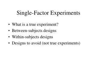
One Factor Experiments • Used to compare alternatives of a single categorical variable For example, several processors, several caching schemes
Example 20.1: Code Size Comparison • Entries in a row are unrelated (Otherwise, need a two factor analysis)
Example 20.1: Interpretation • Average processor requires 187.7 bytes of storage • The effects of the processors R, V, and Z are -13.3, -24.5, and 37.7, respectively. That is, • R requires 13.3 bytes less than an average processor • V requires 24.5 bytes less than an average processor, and • Z requires 37.7 bytes more than an average processor.
Estimating Experimental Errors • Estimated response for jth alternative: • Error: • Sum of squared errors (SSE):
Allocation of Variation (cont’d) • Total variation of y (SST):
Example 20.3 (cont’d) • 89.6% of variation in code size is due to experimental errors (programmer differences) Is 10.4% statistically significant?
Analysis of Variance (ANOVA) • Importance ¹ Significance • Important Explains a high percent of variation • Significance High contribution to the variation compared to that by errors • Degree of freedom = Number of independent values required to compute • Note that the degrees of freedom also add up.
F-Test • Purpose: to check if SSA is significantly greater than SSE • Errors are normally distributed SSE and SSA have chi-square distributions • The ratio (SSA/nA)/(SSE/ne) has an F distribution • where nA=a-1 = degrees of freedom for SSA • ne=a(r-1) = degrees of freedom for SSE • Computed ratio > F[1- a; nA, ne] SSA is significantly higher than SSE. SSA/nA is called mean square of A or (MSA) Similary, MSE=SSE/ne
Computed F-value < F from Table The variation in the code sizes is mostly due to experimental errors and not because of any significant difference among the processors Example 20.4: Code Size Comparison
Visual Diagnostic Tests Assumptions: • Factors effects are additive • Errors are additive • Errors are independent of factor levels • Errors are normally distributed • Errors have the same variance for all factor levels Tests: • Residuals versus predicted response: No trend Independence Scale of errors << Scale of response Ignore visible trends • Normal quantilte-quantile plot linear Normality
Example 20.5 • Horizontal and vertical scales similar Residuals are not small Variation due to factors is small compared to the unexplained variation • No visible trend in the spread • Q-Q plot is S-shaped shorter tails than normal
Confidence Intervals For Effects • Estimates are random variables • For the confidence intervals, use t values at a(r-1) degrees of freedom. • Mean responses: • Contrasts å hjaj: Use for a1-a2
Example 20.6 (cont’d) • For 90% confidence, t[0.95; 12]= 1.782 • 90% confidence intervals: • The code size on an average processor is significantly different from zero • Processor effects are not significant
Example 20.6 (cont’d) • Using h1=1, h2=-1, h3=0, (å hj=0): • CI includes zero one isn't superior to other
Example 20.6 (cont’d) • Similarly, • Any one processor is not superior to another
Unequal Sample Sizes • By definition: • Here, rj is the number of observations at jth level. N =total number of observations:
Example 20.7: Code Size Comparison • All means are obtained by dividing by the number of observations added • The column effects are 2.15, 13.75, and -21.92
Example 20.6 ANOVA (cont’d) • Sums of Squares: • Degrees of Freedom:
Example 20.6 ANOVA Table • Conclusion: Variation due processors is insignificant as compared to that due to modeling errors
Example 20.6 Standard Dev. of Effects • Consider the effect of processor Z: Since, • Error in a3 = å Errors in terms on the right hand side: • eij's are normally distributed a3 is normal with
Summary • Model for One factor experiments: • Computation of effects • Allocation of variation, degrees of freedom • ANOVA table • Standard deviation of errors • Confidence intervals for effects and contracts • Model assumptions and visual tests
Exercise 20.1 • For a single factor design, suppose we want to write an expression for aj in terms of yij's: • What are the values of a..j's? From the above expression, the error in aj is seen to be: • Assuming errors eij are normally distributed with zero mean and variance se2, write an expression for variance of eaj. Verify that your answer matches that in Table 20.5.
An Example Analyze the following one factor experiment: • Compute the effects • Prepare ANOVA table • Compute confidence intervals for effects and interpret • Compute Confidence interval for a1-a3 • Show graphs for visual tests and interpret