Download
1 / 37
370 likes | 586 Vues
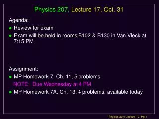
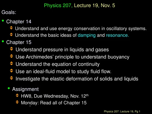
Physics 207, Lecture 19, Nov. 8. Ch. 14: Fluid flow Ch. 15: Oscillatory motion Linear oscillator Simple pendulum Physical pendulum Torsional pendulum. Agenda: Chapter 14, Finish, Chapter 15, Start . Assignments: Problem Set 7 due Nov. 14, Tuesday 11:59 PM

E N D
Physics 207, Lecture 19, Nov. 8 • Ch. 14: Fluid flow • Ch. 15: Oscillatory motion • Linear oscillator • Simple pendulum • Physical pendulum • Torsional pendulum • Agenda: Chapter 14, Finish, Chapter 15, Start Assignments: • Problem Set 7 due Nov. 14, Tuesday 11:59 PM • For Monday, Finish Chapter 15, Start Chapter 16
Fluids in Motion • Up to now we have described fluids in terms of their static properties: • Density r • Pressure p • To describe fluid motion, we need something that can describe flow: • Velocity v • There are different kinds of fluid flow of varying complexity • non-steady/ steady • compressible / incompressible • rotational / irrotational • viscous / ideal
Types of Fluid Flow • Laminar flow • Each particle of the fluid follows a smooth path • The paths of the different particles never cross each other • The path taken by the particles is called a streamline • Turbulent flow • An irregular flow characterized by small whirlpool like regions • Turbulent flow occurs when the particles go above some critical speed
Types of Fluid Flow • Laminar flow • Each particle of the fluid follows a smooth path • The paths of the different particles never cross each other • The path taken by the particles is called a streamline • Turbulent flow • An irregular flow characterized by small whirlpool like regions • Turbulent flow occurs when the particles go above some critical speed
Onset of Turbulent Flow The SeaWifS satellite image of a von Karman vortex around Guadalupe Island, August 20, 1999
streamline Ideal Fluids • Fluid dynamics is very complicated in general (turbulence, vortices, etc.) • Consider the simplest case first: the Ideal Fluid • No “viscosity” - no flow resistance (no internal friction) • Incompressible - density constant in space and time • Simplest situation: consider ideal fluid moving with steady flow - velocity at each point in the flow is constant in time • In this case, fluid moves on streamlines
streamline Ideal Fluids • Streamlines do not meet or cross • Velocity vector is tangent to streamline • Volume of fluid follows a tube of flow bounded by streamlines • Streamline density is proportional to velocity • Flow obeys continuity equation Volume flow rate Q = A·vis constant along flow tube. Follows from mass conservation if flow is incompressible. A1v1 = A2v2
(A) 2 v1 (B) 4 v1 (C) 1/2 v1 (D) 1/4 v1 Lecture 19Exercise 1Continuity v1 • A housing contractor saves some money by reducing the size of a pipe from 1” diameter to 1/2” diameter at some point in your house. v1/2 • Assuming the water moving in the pipe is an ideal fluid, relative to its speed in the 1” diameter pipe, how fast is the water going in the 1/2” pipe?
DV Conservation of Energy for Ideal Fluid • Recall the standard work-energy relation W = DK = Kf - Ki • Apply the principle to a section of flowing fluid with volume DV and mass Dm = r DV (here W is work done on fluid) • Net work by pressure difference over Dx (Dx1 = v1Dt) • Focus first on W = F Dx W = F1Dx1 – F2Dx2 = (F1/A1) (A1Dx1) – (F2/A2) (A2Dx2) = P1DV1 – P2DV2 and DV1 = DV2 = DV (incompressible) W = (P1– P2 ) DV Bernoulli Equation P1+ ½ r v12 + r g y1 = constant
DV Conservation of Energy for Ideal Fluid • Recall the standard work-energy relation W = DK = Kf - Ki W = (P1– P2 ) DV and W = ½ Dm v22 – ½ Dm v12 = ½ (rDV) v22 – ½ (rDV)v12 (P1– P2 ) = ½ r v22 – ½ r v12 P1+ ½ r v12= P2+ ½ r v22= constant (in a horizontal pipe) Bernoulli Equation P1+ ½ r v12 + r g y1 = constant
(A) smaller (B) same (C) larger Lecture 19Exercise 2Bernoulli’s Principle v1 • A housing contractor saves some money by reducing the size of a pipe from 1” diameter to 1/2” diameter at some point in your house. v1/2 2) What is the pressure in the 1/2” pipe relative to the 1” pipe?
Applications of Fluid Dynamics • Streamline flow around a moving airplane wing • Lift is the upward force on the wing from the air • Drag is the resistance • The lift depends on the speed of the airplane, the area of the wing, its curvature, and the angle between the wing and the horizontal higher velocity lower pressure lower velocity higher pressure Note: density of flow lines reflects velocity, not density. We are assuming an incompressible fluid.
Back of the envelope calculation • Boeing 747-400 • Dimensions: • Length: 231 ft 10 inches • Wingspan: 211 ft 5 in • Height: 63 ft 8 in • Weight: • Empty: 399, 000 lb • Max Takeoff (MTO): 800, 000 lb • Payload: 249, 122 lb cargo • Performance: • Cruising Speed: 583 mph • Range: 7,230 nm • r (v22- v12) / 2 = P1 – P2 = DP Let v2 = 220.0 m/s v2 = 210 m/s So DP = 3 x 10³ Pa = 0.03 atm or 0.5 lbs/in2 http://www.geocities.com/galemcraig/ Let an area of 200 ft x 15 ft produce lift or 4.5 x 10⁵ in2 or just 2.2 x 10⁵ lbs upshot Downward deflection Bernoulli (a small part) Circulation theory
Venturi Bernoulli’s Eq.
Cavitation Venturi result In the vicinity of high velocity fluids, the pressure can gets so low that the fluid vaporizes.
k m k m k m Chapter 15Simple Harmonic Motion (SHM) • We know that if we stretch a spring with a mass on the end and let it go the mass will oscillate back and forth (if there is no friction). • This oscillation is called Simple Harmonic Motion and if you understand a sine or cosine is straightforward to understand.
F= -k x a k m x SHM Dynamics • At any given instant we know thatF= mamust be true. • But in this case F= -k x and ma= • So: -k x = ma = a differential equation for x(t) ! Simple approach, guess a solution and see if it works!
SHM Solution... • Eithercos ( t)orsin ( t)can work • Below is a drawing of A cos ( t) • where A=amplitude of oscillation T = 2/ A A
SHM Solution... • What to do if we need the sine solution? • Notice A cos(t + )= A [cos(t) cos() - sin(t) sin() = [A cos()] cos(t) - [A sin()] sin(t) = A’cos(t) + A” sin(t) (sine and cosine) • Drawing of A cos(t + )
SHM Solution... • Drawing of A cos (t -/2) A = A sin( t )
What about Vertical Springs? • For a vertical spring, if yis measured from the equilibrium position • Recall: force of the spring is the negative derivative of this function: • This will be just like the horizontal case:-ky = ma = j k y = 0 F= -ky m Which has solution y(t) = A cos( t + ) where
by taking derivatives, since: xmax = A vmax = A amax = 2A k m x 0 Velocity and Acceleration Position: x(t) =A cos(t + ) Velocity: v(t) = -A sin(t + ) Acceleration: a(t) = -2A cos(t + )
Lecture 19, Exercise 3Simple Harmonic Motion • A mass oscillates up & down on a spring. It’s position as a function of time is shown below. At which of the points shown does the mass have positive velocity and negative acceleration ? Remember: velocity is slope and acceleration is the curvature y(t) (a) (c) t (b)
k m x Example • A mass m = 2 kg on a spring oscillates with amplitude A = 10cm. At t = 0its speed is at a maximum, and is v=+2 m/s • What is the angular frequency of oscillation ? • What is the spring constant k ? General relationships E = K + U = constant, w = (k/m)½ So at maximum speed U=0 and ½ mv2 = E = ½ kA2 thus k = mv2/A2= 2 x (2) 2/(0.1)2 = 800 N/m, w = 20 rad/sec
k m x 0 Initial Conditions Use “initial conditions” to determine phase! sin cos
m Lecture 19, Example 4Initial Conditions • A mass hanging from a vertical spring is lifted a distance dabove equilibrium and released at t = 0. Which of the following describe its velocity and acceleration as a function of time (upwards is positive y direction): (A) v(t) = - vmax sin( wt ) a(t) = -amax cos( wt ) k y (B) v(t) = vmaxsin( wt ) a(t) = amax cos( wt ) d t = 0 (C) v(t) = vmaxcos( wt ) a(t) = -amax cos(wt ) 0 (both vmax and amax are positive numbers)
x(t) = A cos( t + ) v(t) = -A sin( t + ) a(t) = -2A cos(t + ) Energy of the Spring-Mass System We know enough to discuss the mechanical energy of the oscillating mass on a spring. Remember, Kinetic energy is always K = ½ mv2 K = ½ m [ -A sin( t + )]2 And the potential energy of a spring is, U = ½ k x2 U = ½ k [ A cos (t + ) ]2
E = ½ kA2 U~cos2 K~sin2 Energy of the Spring-Mass System Add to get E = K + U = constant. ½ m ( A )2 sin2( t + )+1/2 k (A cos( t + ))2 Remember that so,E = ½ k A2 sin2(t + ) + ½ kA2 cos2(t + ) = ½ k A2 [ sin2(t + ) + cos2(t + )] = ½ k A2 Active Figure
SHM So Far • The most general solution isx = A cos(t + ) where A = amplitude = (angular) frequency = phase constant • For SHM without friction, • The frequency does notdepend on the amplitude ! • We will see that this is true of all simple harmonic motion! • The oscillation occurs around the equilibrium point where the force is zero! • Energy is a constant, it transfers between potential and kinetic.
The Simple Pendulum • A pendulum is made by suspending a mass m at the end of a string of length L. Find the frequency of oscillation for small displacements. S Fy = mac = T – mg cos(q) = m v2/L S Fx = max = -mg sin(q) If q small then x L q and sin(q) q dx/dt = L dq/dt ax = d2x/dt2 = L d2q/dt2 so ax = -g q = L d2q / dt2 L d2q / dt2 - g q = 0 and q = q0 cos(wt + f) or q = q0 sin(wt + f) with w = (g/L)½ z y L x T m mg
The Rod Pendulum • A pendulum is made by suspending a thin rod of length L and mass M at one end. Find the frequency of oscillation for small displacements. S tz = I a = -| r x F | = (L/2) mg sin(q) (no torque from T) -[ mL2/12 + m (L/2)2 ] a L/2 mg q • -1/3 L d2q/dt2 = ½ g q • The rest is for homework… z T x CM L mg
where = 0 cos(t + ) General Physical Pendulum • Suppose we have some arbitrarily shaped solid of mass M hung on a fixed axis, that we know where the CM is located and what the moment of inertia I about the axis is. • The torque about the rotation (z) axis for small is (sin ) = -MgR sinq-MgR z-axis R x CM Mg
wire I Torsion Pendulum • Consider an object suspended by a wire attached at its CM. The wire defines the rotation axis, and the moment of inertia I about this axis is known. • The wire acts like a “rotational spring”. • When the object is rotated, the wire is twisted. This produces a torque that opposes the rotation. • In analogy with a spring, the torque produced is proportional to the displacement: = - kwherek is the torsional spring constant • w = (k/I)½
F = -kx wire a k m x I = 0 cos( t + ) Reviewing Simple Harmonic Oscillators • Spring-mass system • Pendula • General physical pendulum • Torsion pendulum where z-axis x(t) = A cos(t + ) R x CM Mg
U K E U x -A 0 A Energy in SHM • For both the spring and the pendulum, we can derive the SHM solution using energy conservation. • The total energy (K + U) of a system undergoing SMH will always be constant! • This is not surprising since there are only conservative forces present, hence energy is conserved.
U K E U x -A 0 A SHM and quadratic potentials • SHM will occur whenever the potential is quadratic. • For small oscillations this will be true: • For example, the potential betweenH atoms in an H2 molecule lookssomething like this: U x
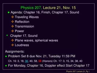
Lecture 19, Recap • Ch. 14: Fluid flow • Ch. 15: Oscillatory motion • Linear spring oscillator • Simple pendulum • Physical pendulum • Torsional pendulum • Agenda: Chapter 14, Finish, Chapter 15, Start Assignments: • Problem Set 7 due Nov. 14, Tuesday 11:59 PM • For Monday, Finish Chapter 15, Start Chapter 16