Download
1 / 17
170 likes | 195 Vues
Assessing benefits of high-resolution models in predicting severe flooding events through a modified sign-test statistic. Comparing radar and gauge data for accuracy. Concluding remarks on scale-intensity analyses and the use of radar fields.

E N D
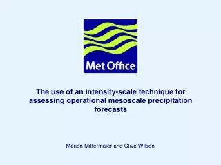
The use of an intensity-scale technique for assessing operational mesoscale precipitation forecasts Marion Mittermaier and Clive Wilson
Outline • An intensity-scale technique (Casati et al. 2004) • Model output and data description • Value added by higher resolution for a severe flooding event (Boscastle, August 2004) • A modified sign-test statistic for highlighting persistent/prevalent errors at the monthly time scale. • Radar vs gauge as “truth” • Concluding remarks
1. An intensity-scale technique ….. best illustrated with an example …. (from Casati, 2004)
Radar Model forecast Radar > 1 mm Forecast > 1 mm Binary error image from Casati (2004)
MSE skill score 1 0 -1 -2 -3 -4 spatial scale (km) Axes multiples of 2 threshold (mm/h) [from Casati (2004)]
2. Model output and data description • Mesoscale version of the Unified Model (MES) runs 4 times a day at ~12 km over the UK (for Unified Model description see Davies et al., QJRMS, 2005) • Newly implemented 4-km model now runs twice a day over the UK (see Bornemann et al, this conference) • Radar-rainfall accumulations available on a 5 km x 5 km national grid • ~2700 rain gauges have been used to produce a daily gridded rainfall product also on a 5 km x 5 km grid
3. Boscastle: the benefit of higher resolution? On 16.08.2004 over 180 mm were recorded by one gauge in a 5-hr period during a highly localised flooding event. How does one assess added benefit? • Output from the MES and 4 km model isn’t directly comparable • Basis of comparison should ideally be the same. Solution: Average the 4 km model output to the 12 km grid and compare against the same 12-km averaged radar rainfall product. …. consider 6-hr rainfall between 12-18Z from the 00Z run …
4 km 00Z 6 hr rainfall MES 00Z 6 hr rainfall 4 km 00Z avg 6 hr rainfall Max radar = 44 mm 46 mm 68 mm 7 mm 12-18Z 12-18Z 12-18Z 16Dx 16Dx Error scale (km) 2Dx 2Dx 1 mm 64 mm Rainfall threshold (mm)
4. A modified sign-test statistic • Distribution-free test as normality of errors can’t be assumed. • B = number of +ve skill scores for a given scale and intensity during a given time interval, e.g. 1 month. • Hypotheses: • H0 : SS >= 0 (implicit positive and skillful) • H1 : SS < 0 (less skill than a random forecast) • H0is rejected if b <= bn,awhere B ~ bi(n, 0.5) for small samples (n < 40), a = 0.025 • The value of (n – B) / n is shaded in intensity-phase space for each scale and intensity where H0 is rejected.
Added benefit: comparison of prevalent errors at the monthly time scale May 2005 MES vs radar May 2005 4 km avg vs radar 32 mm X 48 km X X X X X X X X X X X X X X X X X X X X X • (sub-)“grid” scale errors are more prevalent at trace rainfall totals for the 4 km model • prevalent errors at twice and four times the MES grid length for thresholds > 16 mm are less for the 4 km model (captures large totals better)
5. Radar vs gauge as “truth” August 2004 MES vs radar August 2004 MES vs gauge X X X X X X X X X X X X X X X X X X X X X X • Slight shifts in the distribution of prevalent errors at the monthly time scale • Overall pattern very similar • Radar-rainfall fields preferred as they are truly spatial with a greater observation frequency
6. Concluding remarks • The 4 km model contains much more detail (even when averaged to 12 km) • Detail does not necessarily equal accuracy! Raw model output needs to be averaged • Scale-intensity analyses show that the need for averaging is (almost) independent of grid length (there is always grid noise, regardless) • The difference between error analyses produced using radar (true spatial) and gauge (point-interpolated) fields is minimal. Recommend that radar fields are used also because of the high observation frequency.
MES 12Z 6 hr rainfall Radar 12Z 6 hr rainfall 4 km 12Z avg 6 hr rainfall 12-18Z 12-18Z 12-18Z 19 June 2005 Flash flooding caused by thunderstorms over North Yorkshire Error scale (km) Rainfall threshold (mm)
Haar Wavelet filter deviation from mean value mean value + + mean value on all the domain Casati et al., 2004, Met Apps
An intensity-scale technique using wavelets Haar mother wavelety 1 -1 0 1 2 4 n n+1 • Wavelets are locally defined real functions characterised by a location and a spatial scale. • Any real function can be expressed as a linear combination of wavelets, i.e. as a sum of components with different spatial scales. • Wavelet transforms deal with discontinuities better than Fourier transforms do
wavelet decomposition of the binary error Scale 1 0 -1 from Casati (2004)