Download
1 / 49
490 likes | 620 Vues
This talk by Beate Heinemann from the University of Liverpool discusses ongoing searches for new physics phenomena at the Tevatron, focusing on various signatures and models that go beyond the Standard Model, including SUSY particles, Higgs bosons, and more. Key experimental strategies involve optimizing cuts, understanding background predictions, and applying control regions to ensure data integrity. Attention is given to sophisticated examples such as the search for Bs→mm decays and trilepton signatures, highlighting the challenges researchers face in detecting these phenomena.

E N D
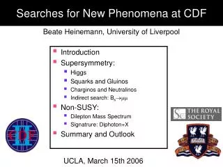
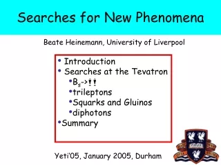
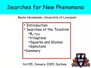
Searches for New Phenomena • Introduction • Searches at the Tevatron • Bs->mm • trileptons • Squarks and Gluinos • diphotons • Summary Beate Heinemann, University of Liverpool Yeti’05, January 2005, Durham
Beyond the Standard Model • Many things to be discovered? • SUSY particles • Non-SM Higgs bosons • Large Extra Dimensions • New Gauge bosons (Z’, W’) • Leptoquarks • Technicolor particles • Others? • Experiments need to be open and cover any possible signature (as manpower allows)! B. Heinemann, University of Liverpool
Cover “all” signatures… • New Physics Models are good for: • Benchmarking and comparing to other experiments • helping theorists to further develop models • Gudiance on experimental signature, choice of cuts etc. • But, should not be too biased towards them • Experimentally we should try to find anything, independently of whether predicted or not • Who knows what may be out there! • Trying to cover ALL experimental signatures (usually you can always find a model that fits it): • Not trivial, large combinatorics with e,m,t,,v,j,b,c and e.g. 6-object final states! • Manpower limited B. Heinemann, University of Liverpool
SUSY: mSugra inspired Covered in this talk Over 60 searches ongoing at both CDF and D0! Ongoing in CDF B. Heinemann, University of Liverpool
How to Search for New Physics • Find favourite model/signature: make MC • Try to define “control regions” to get confidence in background estimates • Optimise cuts to maximise sensitivity • maximise parameter space • choose simple/intuitive cuts as much as possible • Compare data to SM prediction • Derive limit on cross section x BR • Interpret data in your model, best close to what you are searching for: e.g. not M0, M1/2 but rather m(squark) B. Heinemann, University of Liverpool
How to do a Search? (example) • Example: BR(Bs->mm) • Need to: • Know the background: Bgd • Know the acceptance and efficiency: a and e • Know the Bs production cross section sBs • Know uncertainties on those • This case: “blind” • Signal/Blind region: |m(mm)-m(Bs)|<100 MeV,ct>0 • “Side band” region: |m(mm)-m(Bs)|>100 MeV,ct<0 • Understand background from side bands • Understand signal from MC • Don’t look at data until the end=> “blind” B. Heinemann, University of Liverpool
Cut Optimisation • Select ≈3000 events with • 2 muons with pt>2 GeV • Pt(mm)>6 GeV • 4.669<M(mm)<5.969 GeV • Discriminant variables: • Dimuon mass • Lifetime: ct • Df between muons • Isolation of Bs • Cuts optimised to yield maximal Signal/√Bgd B. Heinemann, University of Liverpool
Background Prediction • Background: • Random muons from cc and bb • QCD jets -> pion/kaon->mu+X • Cannot estimate using MC => use “side bands” • Define control regions • Same sign muons • Lifetime<0 (due to misreconstruction) • Get confidence in background prediction! B. Heinemann, University of Liverpool
Signal Acceptance • Does MC reproduce cut variables? • Use B+->J/psi+K+ as control sample • E.g. test isolation cut of Iso>0.65 • MC reproduces J/Psi data well • Assign 5% syst. Error on MC modelling Final upshot: Bgd: 1.1+/-0.3 events => Let’s open the blind box! B. Heinemann, University of Liverpool
Opening the “Box”: Bs->mm :-( Too bad! But nevermind, I can constrain new physics then! B. Heinemann, University of Liverpool
Calculating a limit Different methods: Bayes Frequentist … Source of big arguments amongst statisticians: Different method mean different things Say what YOU have done There is no “right” way Treatment of syst. Errors somewhat tricky But basically: Calculate probability that data consistent with bgd+new physics: P=e-mmN/N! N = observed events m is NBG + Nnew P=5% => 95% CL upper limit on N and thus sxBR=N/(aL) E.g.: 0 events observed means <2.7 events at 95%C.L. B. Heinemann, University of Liverpool
Trileptons vs Bs->mm A. Dedes, H. Dreiner, U. Nierste, P. Richardson BR(Bs)=1x10⁻⁷ BR(Bs)=1x10⁻⁸ Trileptons: 2 fb-1 B. Heinemann, University of Liverpool
Trileptons • Trileptons (e.g. pp->e+e-m+vm): • Result from chargino and neutralino decays • Sensitive to low tanb (else t’s dominate which are harder) • Negative interference between t-channel and s-channel diagrams • Two competing effects: • Cross section largest of squark mass large • BR to leptons largest if slepton mass low Current analysis: M0=75 GeV, M12=175 GeV B. Heinemann, University of Liverpool
Et 3 leptons + • Challenge: • sxBR low (<0.5 pb) • Backgrounds large • Selection • eel, mml, eml (l=isol. track) • Significant Et • Topological cuts B. Heinemann, University of Liverpool
3-lepton result • Combined result: • sxBR<0.3-0.4 pb • Theory comparison • mSugra: m(c±)>97 GeV • tanb=3, A0=0, m>0 • M(c±)≈M(c02)≈2M(c01) • Heavy squarks: m(c±)>111 GeV • Reduce destructive interference • Large m0: • Sleptons heavy • Very difficult L=147-249 pb-1 97 GeV 111 GeV Will extend sensitivity to mSUGRA beyond LEP with just 25% more data: Factor two more already on tape! B. Heinemann, University of Liverpool
Missing Et • Most difficult experimental quantity! • Sources: • Genuine due to n,c (wanted) • Instrumental (unwanted): • Cosmic and beam halo muons showering in calorimeter • Noise • Beam splashes into detector • Mismeasured jets • Uninstrumented parts (cracks) in detector Before Cuts After Cuts • At high Et mostly junk! • Removed by cuts, e.g. • Track towards jet • Beam halo filters • Cosmic filters, timing cuts • etc. B. Heinemann, University of Liverpool
Bottom Squarks • High tanb scenario: • Sbottom could be “light” • This analysis: • Gluino rather light: 200-300 GeV • BR(g->bb)~100% assumed • Spectacular signature: • 4 b-quarks + Et • Require b-jets and Et>80 GeV • Again “blind” analysis • define control regiosn to check backgrounds ~ ~ • Backgrounds: • QCD bb + fake Et • EWK backgrounds: • Wbb->lvbb (l=e,m,t) • Zbb->vvbb • Top background: • tt->lvjjbb • tt->jjjjbb B. Heinemann, University of Liverpool
Control of Backgrounds B. Heinemann, University of Liverpool
Bottom Squarks • Result for 2 b-jets: • Expect 2.6 +- 0.7 events • Observe: 4 events • Data consistent with expectation • Derive limit on cross sectionxBR • Derive limit on sbottom and gluino masses B. Heinemann, University of Liverpool
Light Stop-Quark: Motivation • If stop is light: decay only via t->cc10 • E.g. consistent with relic density from WMAP data • hep-ph/0403224 (Balazs, Carena, Wagner) • WCDM=0.11+-0.02 • M(t)-M(c10)≈15-30 GeV • Search for 2 charm-jets and large Et: • Et(jet)>35, 25 GeV • Et>55 GeV B. Heinemann, University of Liverpool
Light Stop-Quark: Result • Data consistent with background estimate • Observed: 11 • Expected: 8.3+2.3-1.7 • Main background: • Z+ jj -> vvjj • W+jj -> tvjj • Systematic error large: ≈30% • ISR/FSR: 23% • Stop cross section: 16% • Not quite yet sensitive to cross section B. Heinemann, University of Liverpool
Candidate Events D0 squark/gluino cand.: Et=375 GeV!!! CDF stop cand.: Et=53 GeV, 2 charm-jets B. Heinemann, University of Liverpool
Quasi-stable Stop Quarks • Model: • any charged massive particle (e.g. stop, stau) with long lifetime: “quasi-stable” • Assume: fragments like b-quark • Signature • Use Time-Of-Flight Detector: • RTOF ≈140cm • Resolution: 100ps • Heavy particle=> v<<c • DtTOF =ttrack-tevent = 2-3 ns • Result for DtTOF >2.5 ns: • expect 2.9±3.2, observe 7 • s<10-20pb at m=100 GeV • M(t)>97-107 GeV @ 95%C.L. DtTOF ~ m(stop) LEP: 95 GeV B. Heinemann, University of Liverpool
High Mass Dileptons and Diphotons Standard Model high mass production: • Tail enhancement: • Large Extra Dimensions: Arkani-Hamed, Dimopoulos, Dvali (ADD) • Contact interaction New physics at high mass: • Resonance signature: • Spin-1: Z’ • Spin-2: Randall-Sundrum (RS) Graviton • Spin-0: Higgs B. Heinemann, University of Liverpool
Di-Photon Cross Section • Select 2 photons with Et>13 (14) GeV • Statistical subtraction of BG (mostly p0): • Hard to control • MC cannot be trusted • Measure in data • Data agree well with NLO (DIPHOX, RESBOS) • PYTHIA describes shape (but normalisation off by factor 2) Mgg (GeV) B. Heinemann, University of Liverpool
Non-SM Light H Some extensions of SM contain Higgs w/ large B(H) Fermiophobic Higgs : does not couple to fermions Topcolor Higgs : couples to only to top (i.e. no other fermions) Important discovery channel at LHC Event selection 2 Isolated ’s with pT > 25 GeV ||<1.05 (CC) or 1.5<||<2.4 (EC) pT () > 35 GeV (optimised) BG: mostly jets faking photons Syst. error about 30% per photon! Estimated from Data ∫Ldt=191 pb-1 Central-Central Central-Forward B. Heinemann, University of Liverpool
Non-SM Light Higgs H Perform counting experiments on optimized sliding mass window to set limit on B(H) as function of M(H) B. Heinemann, University of Liverpool
Randall-Sundrum Graviton • Analysis: • D0: combined ee and gg • CDF: separate ee, mm and gg • Data consistent with background • Relevant parameters: • Coupling: k/MPl • Mass of 1st KK-mode • World’s best limit from D0: • M>785 GeV for k/MPl=0.1 345 pb-1 B. Heinemann, University of Liverpool
Summary • Search for New Physics is tricky: • Backgrounds: estimate from data and MC • Acceptance: find calibration channels • Control both wherever you can • Beware of BG cross section (NLO, NNLO corrections) • Publish cross section limit (not just exclusion plane) • Illustrated just a few results at Tevatron: • Many more existing (www-cdf.fnal.gov and www-d0.fnal.gov) • Many results from HERA, LEP, BaBar/Belle, etc. • Use models for benchmarking but don’t take them as “truth” • Not found anything yet BUT • it’s a lot of fun • prospects are good! B. Heinemann, University of Liverpool
~ Generic Squarks and Gluinos Et Et • Signature: • 2 jets and • ∑Ptjet > 275 GeV • >175 GeV • Observe: 4, Expect: 2.7±1.0 • mSugra • Fix: m0=25 GeV, tanb=3, A0=0,m<0 • Exclude: m(q/g) < 292/333 GeV • Improves Run I limits: • Include more data • Scan parameter space QCD jets ~ ~ B. Heinemann, University of Liverpool
Neutral Spin-1 Bosons: Z’ • 2 high-Pt electrons, muons, taus • Data agree with BG (Drell-Yan) • Interpret in Z’ models: • E6-models: y, h, c, I • SM-like couplings (toy model) B. Heinemann, University of Liverpool
Dirac Magnetic Monopole • Bends in the wrong plane( high pt) • Large ionization in scint (>500 Mips!) • Large dE/dx in drift chamber TOF trigger designed specifically for monopole search mmonopole > 350 GeV/c2 B. Heinemann, University of Liverpool
Neutral Spin-1 Bosons: Z’ • 95% C.L. Limits for SM-like Z’ (in GeV): Combined CDF limit: M(Z’)>815 GeV/c2 B. Heinemann, University of Liverpool
MSSM Higgs A-> tt • Fit “visible” mass: from leptons, tau’s and Et • Limit on sxBR≈10-2 pb • Interpretation soon in tanb vs mA plane: also sensitive to bbf process B. Heinemann, University of Liverpool
MSSM Higgs: A -> tt • t’s are tough! • Select di-t events: • 1 lepton from tl • 1 hadronic t-decay (narrow jet) • Efficiency ≈1% • Background: mostly Z->tt B. Heinemann, University of Liverpool
MSSM Higgs CDF Run I 95% C.L. • Standard Model: • s(bbH) =1-10 fb: 100 x smaller than WH • In MSSM the bbF (F=A,H) Yukawa coupling grows like tanb: • Larger cross sections • Better discovery potential than SM • Search for final states: • F+b+X->bbb+X • F+X->tt+X • E.g. for M(A)=120 GeV: • 5s discovery for tanb>30 • 3s evidence for tanb>20 S. Willenbrock B. Heinemann, University of Liverpool
D0: Neutral Higgs at High Tan • Event Selection: • At least 3 jets:ET cuts on jets optimized for different Higgs mass values • B-tagging for each jet • Main Background: • QCD multi b-production • Difficult for LO MC: determined from data and/or ALPGEN 1.2 • Signal acceptance about 0.2-1.5% depending on Mass • Result much worse than CDF Run 1!?! • Thought to be due to pdf’s: CTEQ3 vs CTEQ5 ∫Ldt=131 pb-1 B. Heinemann, University of Liverpool
GMSB: gg+Et • Assume c01 is NLSP: • Decay to G+g • G light M~O(1 keV) • Inspired by CDF eegg+Et event: now ruled out by LEP • D0 (CDF) Inclusive search: • 2 photons: Et > 20 (13) GeV • Et > 40 (45) GeV ~ ~ B. Heinemann, University of Liverpool
pp-> bbA ->bbbb Why D0 so much worse with more data??? B. Heinemann, University of Liverpool
pp-> bbA ->bbbb Used CTEQ3L Used CTEQ5L CTEQ3L 3 times larger acceptance x cross section! B. Heinemann, University of Liverpool
Photon Fake Rate • Rate of jets with leading meson (pi0, eta) which cannot be distinguished from prompt photons: Depends on • detector capabilities, e.g. granularity of calorimeter • Cuts! • Systematic error about 30-80% depending on Et • Data higher than Pythia and Herwig • Pythia describes data better than Herwig CDF (preliminary result) B. Heinemann, University of Liverpool
Wh Production: Run 2 data • Selection: • W(mn or en) • 2 jets: 1 b-tagged • Search for peak in dijet invariant mass distribution • No evidence => Cross section limit on • Wh->Wbb production • Techni-r ->Techni-p +W B. Heinemann, University of Liverpool
Luminosity Perspectives B. Heinemann, University of Liverpool
CDF: COT Aging Problem Solved! B. Heinemann, University of Liverpool
Silicon Performance See talk by R. Wallny B. Heinemann, University of Liverpool
CDF: B-tagging and tracking See talk by R. Wallny B. Heinemann, University of Liverpool
Z’ -> tt • t’s challenging at hadron colliders: • t signals established by CDF & D0: W->tn, Z->tt • 1- and 3-prong seen • Result for mvis>120 GeV: • Observe: 4 events • Expect: 2.8±0.5 • M(Z’)>395 GeV • Ruled out by ee and mm channel for SM Z’ => explore other models with enhanced t couplings B. Heinemann, University of Liverpool
RPV Neutralino Decay • Model: • R-parity conserving production => two neutralinos • R-parity violating decay into leptons • One RPV couplings non-0: l122 , l121 • Final state: 4 leptons +Et • eee, eem, mme, mmm • 3rd lepton Pt>3 GeV • Largest Background: bb • Interpret: • M0=250 GeV, tanb=5 _ l121>0 l122>0 ~ ~ ~ m(c+1) >160 GeV m(c+1) >183 GeV B. Heinemann, University of Liverpool