Download
1 / 35
370 likes | 717 Vues
Atmospheric Effects on SAR and InSAR. Cameron Lewis EECS 826 Spring 2009. Agenda. Meteorological Review Atmospheric structure and constituents Absorption and scattering Index of refraction Degrading Effects Moving hills Spatially variant defocusing Turbulence-induced distortion

E N D
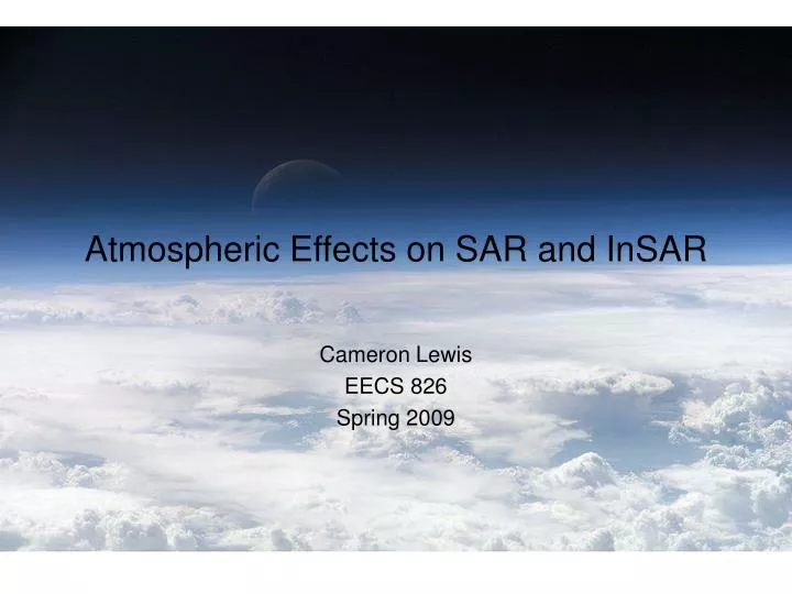
Atmospheric Effects on SAR and InSAR Cameron Lewis EECS 826 Spring 2009
Agenda • Meteorological Review • Atmospheric structure and constituents • Absorption and scattering • Index of refraction • Degrading Effects • Moving hills • Spatially variant defocusing • Turbulence-induced distortion • Tropospheric range delay • Other influences • Mitigation Techniques • Atmospheric structure extraction using SAR
Meteorological Review Temperature Structure: • Troposphere: • Where the weather occurs • Lapse rate: 6.8°C/km • Water vapor • Dynamically layered: • Boundary layer (ABL) • Ekman layer • Free atmosphere (FA) • Stratosphere • Mesosphere • Thermosphere
Meteorological Review Planetary Boundary Layer [1]:
Meteorological Review Radiosonde SkewT-LogP plot for Albuquerque, NM (1 Apr 2004) Note significant drop in dew point starting at 600 mb = Top of ABL Corresponding altitude: ~4km
Meteorological Review Ekman Layer: • Hypothetical layer at the base of the FA • Does not exist in Earth’s troposphere due to it’s statistically stable nature • Weak, shallow Ekman spirals can exist under the right conditions (rare) Free Atmosphere: • Insulated from the surface by the ABL capping inversion • Treated (dynamically) as an ideal fluid • Typically follows the standard tropospheric models
Meteorological Review Ionosphere: • Characterized by significant concentration of electrons and ions • Starts at roughly 45 miles • Often divided into regions based on local maxima and influence: • D region • E layer • Sporadic-E clouds • F layer
Meteorological Review Pressure Structure: • Standard dry atmosphere, decreases with altitude: P(z) = 2.87ρair(z)T(z) where ρ is dry air density as defined for a standard atmosphere below 30 km • Helps define troposphere and tropospheric layers.
Meteorological Review Atmospheric Constituents (by volume): • Permanent Gases: • Nitrogen 78.08% • Oxygen 20.95% • Argon 0.93% • Neon 0.0018% • Variable Gases: • Water Vapor 0 to 4% • Carbon Dioxide 0.037% • Methane 0.00017% • Nitrous Oxide 0.00003% • Ozone 0.000004% Highly variable, especially within the ABL. Sharp changes lead to sharp gradients in the index of refraction.
Meteorological Review Absorption • Primarily occurs in known frequency bands • Primarily due to oxygen and water vapor • Oxygen: 60 GHz complex and 118.75 GHz • Water vapor: 22.235 GHz • Manifests as attenuation Scattering • Due to the presence of objects within the signal path • i.e.: hydrometeors, pollutants, etc • Manifests as attenuation
Meteorological Review Index of Refraction • Defines the change in the speed of light within a medium • Causes bending of wavefront vector • Atmospheric index of refraction dependent on temperture and dew point (humidity) • Note: parabolic distribution of refractive index can cause lensing
Degrading Effects Moving Hills (observed by Sandia National Laboratories) [2]: • Illustration of phenomena • Initial testing of long-range airborne SAR revealed anomalies in wide-area spotlight images, appeared as uneven illumination • Exhaustive testing to rule out instrument deficiencies (hardware and software)
Degrading Effects Moving Hills: • Images collected at ranges of nearly 100 km and altitudes of 4.5 – 6 km • Clearly show the movement of “hills” in successive images of the exact same scene • Anomalies vary in amplitude from relatively strong to relatively weak • Only change between successive images is the atmospheric path (spotlight mode) • Strong evidence anomaly is associated with a relatively stationary weak atmospheric perturbation
Degrading Effects Sequence of spotlight images exhibiting a “moving hill” (1 April 2004) [2]
Degrading Effects Spatially variant defocusing [2]: • Long-range, fine-resolution images exhibited spatially variant sidelobe structures, the result of spatially variant phase errors • System errors ruled out (as discussed) • Note presence of strong sidelobes • Capture parameters: • Range: 46 km • Altitude: 5.8 km • Resolution: 0.3 m
Degrading Effects Three questions arise: • Can these phenomena be modeled in a fashion that incorporated atmospheric variations? • If so, can the atmosphere even produce the witnessed phenomena? • If so, by what mechanism? Without atmospheric perturbations, SAR data is commonly modeled using a well-established equation:
Degrading Effects For each sampling of the scene along the synthetic aperture (angle α), we assume a small perturbation modifies the illuminated scene by a factor f(x,y;α): Using reciprocity, we can apply this modification through the antenna factor AR as seen above. We also have to account for the modification to the radiation scattered to the antenna by a differential element σ(x,y):
Degrading Effects The definition of the f function can be simple or elaborate. A simple f function can be derived is a simple anomaly geometry is assumed. Moving hills shape suggest a concentration or dispersion of energy reminiscent of a weak lens. This lens effect attainable through bumps along the top of the ABL.
Degrading Effects The focal length of a parabolic lens: Where n1 and n2 indicate the index of refraction just below an above the transition
Degrading Effects The f function can then be defined as: where z is the focal length from the previous slide, R is the range to the target, and the index of refraction n is defined by: where T and Tdp are the absolute and dew point temperatures respectively (in Kelvin)
Degrading Effects So what about our questions? • Can these phenomena be modeled in a fashion that incorporated atmospheric variations? Yes, we can model atmospheric perturbations as modifications to both the antenna pattern and modifications to the target RCS. • If so, can the atmosphere even produce the witnessed phenomena? Yes, the atmosphere is capable of creating lens structure that can focus or disperse energy • If so, by what mechanism? “Via gradients in the index of refraction at the interface to the ABL, due principally to humidity gradients at the interface” [2]
Degrading Effects Turbulence-Induced Distortions [7]: • Well known that turbulence is capable of producing phase errors in SAR imagery (See Porcello [8]) • Consider geometry, mean square two-way phase shift of a plane wave propagating a distance S through a turbulent medium: where L0 is the size of the largest turbulent eddies, and Cn is the index of refraction structure constant (defined by Porcello [8])
Degrading Effects • Mean square phase shifts less than 1 rad2 won’t effect SAR images • Mean square phase shifts greater than 1 rad2 may have significant effects on SAR images • Phase shifts become larger with increasing eddy size and frequency
Degrading Effects • Introduce turbulent layer into typical SAR imaging geometry • Assume all rays travel straight path through turbulence • Turbulent layer imposes an additional phase shift to the signal due to changes in the index of refraction within the layer
Degrading Effects Through rigorous mathematical manipulation, the reflected signal from the surface through the turbulent layer is: where a = h1λR0/2h and Desired Image Distortion introduced by the turbulent layer
Degrading Effects To give this result some meaning, lets assume the image consists of 2 parallel, straight lines separated by a distance b: This produces: Desired Image Blurred line with spread a/L centered at –K0a Blurred line with spread a/L centered at b – K0a
Degrading Effects Tropospheric Range Delay [9]: • Delay due to ionosphere equivalent to dozens of meters • Delay due to troposphere equivalent to a few meters One way range delay determined by: where N is refractivity and γ is satellite elevation As before, N can be determined via: The following accepted parameter expressions may be used:
Degrading Effects Tropospheric Range Delay Correction: • Surface meteorological data collection stations used to determine sea level range delay • Range delay map created • Range delay compared with GPS calculated range delay for verification • Calculated range delay phase was subtracted from the initial interferometric phase • Differential interferogram was created using an estimated baseline
Degrading Effects Additional effects of modified propagation by the atmosphere: • Differential SAR Interferometry (DInSAR) [10] • Remove topography induced phase from InSAR interferograms through an accurate DEM, so as to unveil observed surface displacements. • Process confounded by differing atmospheric phase errors due to long lags between repeat-pass interferometry. • Again, atmospheric turbulence and refractive index gradients due to sharp humidity gradients in the ABL are to blame • Effects of ABL Moisture on Friction Velocity [11] • Friction velocity is strongly dependent on surface moisture • Friction velocity is related to surface roughness • These atmospheric effects are observable in SAR imagery • Important at low wind speeds • Implication: consider contribution of water vapor to static stability with interpreting ocean SAR imagery, especially at low wind speeds
Mitigation Techniques • Proposal: correct anomalies through measurement and characterization (modeling) of ABL • While plausible, proper ABL characterization requires sufficient accuracy and precision that are unlikely attainable • A more attractive mitigation scheme is to correct the images directly • Moving hills [2] • Averaging scheme across multiple spotlight images • Take median value of collocated pixels across multiple images • Schemes for hill mitigation using single images are currently insufficient
Mitigation Techniques • Spatially variant defocusing [2] • Image blurring typically calls upon autofocus algorithms • This assumes that the blurring is sufficiently uniform • Defocusing due to ABL interface does not allow for single focus correction • However, defocus is often sufficiently uniform over regions of the image • Autofocus routines can be used when the image is segmented into subimages, each using their own autofocus routine • Note the regional autofocus applied to the corner reflector image from before: energy formally spread as sidelobes is now concentrated into the mainlobe
Mitigation Techniques Spatially variant defocusing: After applying regional autofocus operation Raw Image
Atmospheric Structure Extraction • Identification of convective updrafts/downdrafts using SAR imagery [12] • Within the marine atmospheric boundary layer (MABL) • Momentum flux within updraft/downdraft couplets is asymmetric • Leads to creation of cm-scale gravity waves on ocean surface • Use of cm-scale sensitive SAR to identify these zones • Anomalies caused by gradients in the index of refraction at the top of the ABL can be used to determine the height of the ABL (under fixed ionospheric conditions)
References [1] Stull, R. B., 1988: An Introduction to Boundary Layer Meteorology. Kluwer Academic, 666 pp. [2] Dickey, F.M., Doerry, A.W., and Romero, L.A., ‘Degrading effects of the lower atmosphere on long-range airborne synthetic aperture radar imaging’. IET Radar Sonar Navig., 2007, 1, pp. 329-339. [3] Carlson, T. N., 1998: Mid-Latitude Weather Systems. American Meteorological Society, Boston, 507 pp. [4] Holton, J. R., 2004: An Introduction to Dynamic Meteorology. Elsevier Academic Press, Boston, 535 pp. [5] Glickman, T. S. Ed., 2000: Glossary of Meteorology. American Meteorological Society, Boston, 855 pp. [6] Stephens, G. L., 1994: Remote Sensing of the Lower Atmosphere. Oxford University Press, New York, 523 pp. [7] Fante, R. L, ‘Turbulence-Induced Distortion of Synthetic Aperture Radar Images’. IEEE Trans. on Geo. and Remote Sens., 1994, 32, pp. 958-961. [8] Porcello, L. J., ‘Turbulence-Induced Phase Errors in Synthetic-Aperture Radars’. IEEE Trans. Aerospace Electron. Syst., 1970, 6, pp. 636-644. [9] Kimura, H., Kinoshita, H., ‘Effect of tropospheric range delay corrections on differential SAR interferograms’. IEEE International Geosciences and Remote Sensing Symposium 2001, 2001, 5, pp. 2049-2051. [10] Di Bisceglie, M., Fusco, A., Galdi, C., and Sansosti, E., ‘Stochastic modeling of atmospheric effects in SAR differential interferometry’. IEEE International Geosciences and Remote Sensing Symposium 2001, 2001, 6, pp. 2677-2679. [11] Babin, S. M., Thompson, D. R., ‘Effects of Atmospheric Boundary Layer Moisture on Friction Velocity with Implications for SAR Imagery’. IEEE Transactions on Geoscience and Remote Sensing, 2000, 38, pp. 618-621. [12] Sikora, T. D., Bleidorn, J. C., and Thompson, D. R., ‘On Extraction of atmospheric structure from synthetic aperture radar imagery’. IEEE International Geosciences and Remote Sensing Symposium 1999, 1999, 4, pp. 1972-1974.