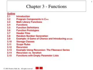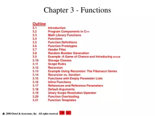
Chapter 3 Functions and Files

1. Chapter 3 Functions and Files

2. 3-2 Getting Help for Functions You can use the lookfor command to find functions that are relevant to your application. For example, type lookfor imaginary to get a list of the functions that deal with imaginary numbers. You will see listed: imag Complex imaginary part i Imaginary unit j Imaginary unit There is also conj(x), real(x), angle(x), abs(x) More? See page 142.

3. Some common mathematical functions: Table 3.1–1 3-3 Exponential; e x Square root; x ( automatically produces imaginary sqrt(-4) = 2*I ) Natural logarithm; ln x Common (base 10) logarithm; log x = log10x (continued…) Exponential exp(x) sqrt(x) Logarithmic log(x) log10(x) In class: T3.1-1 p145

4. Numeric ceil(x) fix(x) floor(x) round(x) sign(x) Round to nearest integer toward ∞. Round to nearest integer toward zero. Round to nearest integer toward -∞. Round toward nearest integer. Signum function: +1 if x >0; 0 if x = 0; -1 if x <0. Some common mathematical functions (continued) >> ceil(1.1) ans = 2 >> fix(1.1) ans = 1 >> floor(1.1) ans = 1 >> floor(-1.1) ans = -2 >> fix(-1.1) ans = -1 >> round(1.1) ans = 1 >> round(-1.1) ans = -1 All of these functions work on vectors element by element, like any other Matlab function 3-5 More? See pages 142-148.

5. The rectangular and polar representations of the complex number a + ib. Figure 3.1–1 3-6

6. Complex Functions x = a + ib abs(x) = sqrt(a^2+b^2) - Absolute value. angle(x) = atan2(b,a) - Angle of a complex number. (note the imaginary part comes 1st) conj(x) = a – ib - Complex conjugate. real(x) = a - Real part of a complex number. imag(x) = b - Imaginary part of a complex number. If x is a complex vector, abs(x) will give you vector of absolute values, not length of a vector Need norm(x) = sqrt(x’*x) 3-4

7. 3-7 Operations with Complex Numbers >>x = -3 + 4i; >>y = 6 - 8i; >>mag_x = abs(x) mag_x = 5.0000 >>mag_y = abs(y) mag_y = 10.0000 >>mag_product = abs(x*y) 50.0000 (continued …)

8. 3-8 Operations with Complex Numbers (continued) >>angle_x = angle(x) angle_x = 2.2143 % radians >>angle_y = angle(y) angle_y = -0.9273 >>sum_angles = angle_x + angle_y sum_angles = 1.2870 >>angle_product = angle(x*y) angle_product = 1.2870 % - same as sum of angles In class: T3.1-2 p145, T3.1-3 p147 More? See pages 143-145.

9. 3-9 Operations on Arrays MATLAB will treat a variable as an array automatically. For example, to compute the square roots of 5, 7, and 15, type >> x = [ 4 49 25] x = 4 49 25 >> y = sqrt(x) y = 2 7 5

10. 3-10 Expressing Function Arguments We can write sin 2 in text, but MATLAB requires parentheses surrounding the 2 (which is called the function argument or parameter). Thus to evaluate sin 2 in MATLAB, we type sin(2). The MATLAB function name must be followed by a pair of parentheses that surround the argument. To express in text the sine of the second element of the array x, we would type sin[x(2)]. However, in MATLAB you cannot use square brackets or braces in this way, and you must type sin(x(2)). (continued …)

11. 3-11 Expressing Function Arguments (continued) To evaluate cos(x 3 -1), you type cos(x.^3 - 1). To evaluate tan(x-2), you type tan(sqrt(x)-2). Using a function as an argument of another function is called function composition. Be sure to check the order of precedence and the number and placement of parentheses when typing such expressions. Every left-facing parenthesis requires a right-facing mate.

12. 3-12 Expressing Function Arguments (continued) Another common mistake involves expressions like cos3x, which means (cos x)3. In MATLAB we write this expression as (cos(x)).^3, NOTas cos^3(x),cos^3x, cos(x^3), or cos(x)^3!

13. 3-13 Expressing Function Arguments (continued) The MATLAB trigonometric functions operate in radian mode. Thus sin(5) computes the sine of 5 rad, not the sine of 5°. To convert between degrees and radians, use the relation qradians = (pi /180)qdegrees. Similarly, inverse trig functions return an answer in radians: asin(0.5) gives 0.5236 radians More? See pages 145-146.

14. Trigonometric functions: Table 3.1–2 3-14 Cosine; cos x. Cotangent; cot x. Cosecant; csc x. Secant; sec x. Sine; sin x. Tangent; tan x. cos(x) cot(x) csc(x) sec(x) sin(x) tan(x)

15. acos(x) acot(x) acsc(x) asec(x) asin(x) atan(x) atan2(y,x) Inverse cosine; arccosx. Inverse cotangent; arccotx. Inverse cosecant; arccscx. Inverse secant; arcsecx. Inverse sine; arcsinx . Inverse tangent; arctanx . Four-quadrant inverse tangent -- see next page. Inverse Trigonometric functions: Table 3.1–2 3-15

16. Difference between atan and atan2 Matlab has two inverse tangent function (see above). atan(x) returns angle between –pi/2 and pi/2. However, another correct answer is the angle that lies on opposite quadrant. atan(1) gives 0.7854 rad  45 degrees But tan(45deg +180deg ) = tan(225deg) = 1 as well Matlab uses atan2(y,x) to determine the arctangent unambiguously. It gives the ange between positive real axis x and line from origin to (x,y) >> atan(1/1) ans = 0.7854 >> atan(-1/-1) ans = 0.7854 >> atan(1/-1) ans = -0.7854 >> atan(-1/1) ans = -0.7854 >> atan2(1,1) ans = 0.7854 >> atan2(-1,-1) ans = -2.3562 >> atan2(-1,1) ans = -0.7854 >> atan2(1,-1) ans = 2.3562 The order of arguments is important for atan2 NOTE that y comes 1st !!!

17. Hyperbolic functions: Table 3.1–3 3-16 Hyperbolic cosine Hyperbolic cotangent. Hyperbolic cosecant Hyperbolic secant Hyperbolic sine Hyperbolic tangent cosh(x) coth(x) csch(x) sech(x) sinh(x) tanh(x)

18. acosh(x) acoth(x) acsch(x) asech(x) asinh(x) atanh(x) Inverse hyperbolic cosine Inverse hyperbolic cotangent Inverse hyperbolic cosecant Inverse hyperbolic secant Inverse hyperbolic sine Inverse hyperbolic tangent; Inverse Hyperbolic functions: Table 3.1–3 3-17

19. User-Defined Functions

20. User-Defined Functions -- must be in a function file (or as a sub-function before or after the main code). Unlike script file, all the variables in function file are local (available only within a function). Functions operate on local variables in their own workspace, separate from Matlab command space. Functions – encapsulate repeated operations. The first line in a function file must begin with a function definitionlinethat has a list of inputs and outputs. This line distinguishes a function M-file from a script M-file. function [output variables] = name(input variables) Note that the output variables are enclosed in square brackets (only need it for more than one output variable), while the input variables must be enclosed with parentheses. In the case that function is stored in a separate file, its name (here, name) should be the same as the file name in which it is saved (with the .m extension). 3-18 More? See pages 148-149.

21. User-Defined Functions: Example function z = fun(x,y) % just one output variable, so do not need [] u = 3*x; z = u + 6*y.^2; % Note: u,z – local variables end Note: u,z – local variables Note the use of a semicolon at the end of the lines. This prevents the values of u and z from being displayed. Note also the use of the array exponentiation operator (.^). This enables the function to accept y as an array. Call this function with its output argument: >>z = fun(3,7) z = 303 The function uses x = 3 and y = 7 to compute z. 3-19

22. 3-21 User-Defined Functions: Example (continued) Call this function without its output argument and try to access its value. You will see an error message. >>fun(3,7) ans = 303 >>z ??? Undefined function or variable ’z’. (continued …)

23. 3-22 User-Defined Functions: Example (continued) Assign the output argument to another variable: >>q = fun(3,7) q = 303 You can suppress the output by putting a semicolon after the function call. For example, if you type q = fun(3,7); the value of q will be computed but not displayed (because of the semicolon).

24. The variables x and y are localto the function fun, so unless you pass their values by naming them x and y, their values will not be available in the workspace outside the function. The variable u is also local to the function. For example, >>x = 3;y = 7; >>q = fun(x,y); >>x x = 3 >>y y = 7 >>u ??? Undefined function or variable ’u’. 3-23

25. 3-24 Only the order of the arguments is important, not the names of the arguments: >>x = 7;y = 3; >>z = fun(y,x) z = 303 The second line is equivalent to z = fun(3,7).

26. 3-25 You can use arrays as input arguments: >>r = fun([2:4],[7:9]) r = 300 393 498 % the result is also an array

27. 3-26 A function may have more than one output. These are enclosed in square brackets. For example, the function circle computes the area A and circumference C of a circle, given its radius as an input argument. function [A, C] = circle(r) A = pi*r.^2; % area C = 2*pi*r; % circumference

28. The function is called as follows, if the radius is 4. >>[A, C] = circle(4) A = 50.2655 C = 25.1327 3-27

29. A function may have no input arguments and no output list. For example, the function show_date computes and stores the date in the variable today, and displays the value of today. function show_date today = date end % date is Matlab internal command giving you the date as a string 3-28

30. Examples of Function Definition Lines 3-29 • One input, one output: • function [area_square] = square(side) • 2. Brackets are optional for one input, one output: • function area_square = square(side) • 3. Three inputs, one output: • function [volume_box] = box(height,width,length) • 4. One input, two outputs: • function [area_circle,circumf] = circle(radius) • 5. No named output: function sqplot(side) • Note that comments can be placed anywhere in the function file, but the lines immediately following function definition are displayed by the help and lookfor commands

31. Function Example function [dist,vel] = drop(g,v0,t); % Computes the distance traveled and the % velocity of a dropped object, % as functions of g, % the initial velocity v0, and % the time t. vel = g*t + v0; dist = 0.5*g*t.^2 + v0*t; displayed as help Used array operation because we expect time t to be a vector (continued …) 3-30

32. Function Example (continued) 1. The variable names used in the function definition may, but need not, be used when the function is called: >>a = 32.2; % here use different names >>initial_speed = 10; >>time = 5; >>[feet_dropped,speed] = . . . drop(a,initial_speed,time) a, initial_speed, and time are different local parameters inside the function drop anyway (continued …) 3-31

33. Function Example (continued) 2. The input variables need not be assigned values outside the function prior to the function call, can just use literal numbers: [feet_dropped,speed] = drop(32.2,10,5) 3. The inputs and outputs may be arrays: [feet_dropped,speed]=drop(32.2,10,[0:1:5]) This function call produces the arraysfeet_dropped and speed, each with six values corresponding to the six values of time in the array time. In class: Ch3 #9, 12 3-32 More? See pages 148-153.

34. The functions above does not have to be saved as a separate file. • You can just save it as subfunction 1st and run it right where. • function temp() • a = 32.2; % here use different names • initial_speed = 10; • time = 5; • [feet_dropped,speed] = drop(a,initial_speed,time) • [feet_dropped,speed]=drop(32.2,10,[0:1:5]) • end • function [dist,vel] = drop(g,v0,t); • % Computes the distance traveled and the • % velocity of a dropped object, as functions of g, • % the initial velocity v0, and the time t. • vel = g*t + v0; • dist = 0.5*g*t.^2 + v0*t; • end

35. Global Variables • The global command declares certain variables global, and therefore their values are available to the basic workspace and to other functions that declare these variables global. • The syntax to declare the variables a, x, and q is • globala x q • Any assignment to those variables, in any function or in the base workspace, is available to all the other functions declaring them global. • Note that it is very easy to change a global variable by mistake and very hard to find this error – use it only for global constants. 3-34 More? See pages 153-156.

36. Global Variables (continue) The proper use of global is for parameters which are common to several functions: global g g = 9.81; ….. ……. vel = velfunct(t,v0) function v = velfunc(t,v0) global g; v = v0 – g*t; Book uses ideal gas and van-der-Waals gas example

37. Finding Zeros of a Function We have used before roots to find roots of polynomials, but it only works for polynomials. For arbitrary function, use the fzero function to find the zero of a function of a single variable, which is denoted by x. As always PLOT FIRST One form of its syntax is: Octave function dummy() x = -4:0.01:4; y = funct1(x); plot(x,y) fzero(@funct1,2) fzero(@funct1,[2,3]) [x,fval,exitflag] = fzero(@funct1,2) grid on end function res = funct1(x) res = cos(x)+sin(x); end -------------------------------------------------------------- >> fzero(@(x) (cos(x)+sin(x)),2) ans = 2.3562 fzero(’function’, x0) where function is a string containing the name of the function, and x0 is a user-supplied guess for the zero. The fzero function returns a value of x that is near x0, or NaN if it fails. It cannot find complex roots ( fzero('x^2+1',0) gives NaN). It identifies only points where the function crosses the x-axis, not points where the function just touches the axis. (Although in the latest version used on fzero('x^2',0) gives 0 as it should) For example, fzero(’cos(x)+sin(x)’,2) returns the value 2.3562. 3-35

38. If x0 is vector or length two, fzero assumes that this is interval where sign of function changes. An error is given if it is NOT true. In this case, we are guaranteed to get a value where function changes sign. >> [x,fval] = fzero('cos(x)+sin(x)',[2,3]) x = 2.3562 fval = 1.1102e-016 % get the value of function at solution x >> [x,fval,exitflag] = fzero('cos(x)+sin(x)',2) x = 2.3562 fval = 1.1102e-016 exitflag = 1 % exitflag > 0 – found zero, exitflag < 0 – no interval was found with sign change Note: fzero finds a point x where function changes sign => if it is continuous, f(x) = 0 It it is discontinous, it may return a discontinous point - fzero('tan(x)',1) gives 1.5708 = pi/2

39. Using fzero with User-Defined Functions To use the fzero function to find the zeros of more complicated functions, it is more convenient to define the function in a function file. For example, if y =x + 2e-x-3, define the following function file: function y = f1(x) y = x + 2*exp(-x) - 3; Octave function y = f1(x) y = x + 2*exp(-x) - 3; end x = fzero(@f1,-0.5) (continued …) 3-36

40. Plot of the function y =x + 2e-x- 3. Figure 3.2–1 PLOT FIRST There is a zero near x = -0.5 and one near x = 3. 3-37 (continued …)

41. Example (continued) To find a more precise value of the zero near x = -0.5, type >>x = fzero(@f1,-0.5) The answer is x = -0.5881. 3-38 More? See pages 156-157.

42. Evaluating input functions Example: We would like to write a function that computes the slope of the line between the two points (a, f (a)) and (b, f (b)). Recall that the slope between these two points is give by m = ( f (b) − f (a) )/ ( b − a ) . function dummy() slope(@functtest,1,2) end % slope.m -compute the slope between (a,f(a)) and (b,f(b)) function m = slope(func,a,b) fa = func(a); fb = func(b); m = (fb-fa)/(b-a); end function res = functtest(x) res = x.^2+1; end

43. From here on – skip in your 1st study Finding the Minimum of a Function The fminbnd function finds the minimum of a function of a single variable, which is denoted by x. fminbnd and fsearchmin are NOT available in Octave, use Maxima One form of its syntax is fminbnd(‘function’, x1, x2) % OR fminbnd(@function, x1, x2) where function is a string containing the name of the function. The fminbnd function returns a value of x that minimizes the function in the closed intervalx1 ≤ x ≤ x2. As always, PLOT FIRST For example, fminbnd(’cos’,0,4) returns the value 3.1416 – approximately pi, where cos reaches min of (-1). 3-39

44. When using fminbnd it is more convenient to define the function in a function file. For example, if y = 1 -xe -x, define the following function file: function y = f2(x) y = 1-x.*exp(-x); To find the value of x that gives a minimum of y for 0 £x £ 5, type >>x = fminbnd(’f2’,0,5) The answer is x = 1. To find the minimum value of y, type y = f2(x). The result is y = 0.6321. Or better use [x,fval,exitflag] = fminbnd(’f2’,0,5) To find max of a function, find min of ( - f(x)) 3-40

45. A function can have one or more localminima and a global minimum. If the specified range of the independent variable does not enclose the global minimum, fminbnd will not find the global minimum. fminbnd may find a minimum that occurs on a boundary. 3-41

46. Plot of the function y = 0.025x 5- 0.0625x 4- 0.333x 3+x 2. Figure 3.2–2 This function has one local and one global minimum. On the interval [1, 4] the minimum is at the boundary: x = 1, while there is local min at x = 3. 3-42

47. To find the minimum of a function of more than one variable, use the fminsearch function. One form of its syntax is fminsearch(’function’, x0) where function is a string containing the name of the function. The vector x0 is a guess that must be supplied by the user. 3-43

48. To minimize the function f = xe-x2- y2, we first define it in an M-file, using the vector x whose elements are x(1) = x and x(2) = y. function f = f4(x) f = x(1).*exp(-x(1).^2-x(2).^2); Suppose we guess that the minimum is near x = y = 0. The session is >>fminsearch(’f4’,[0,0]) ans = -0.7071 0.000 Thus the minimum occurs at x = -0.7071, y = 0. The alternative syntax >>[x,fval,exitflag] = fminsearch(’f4’,[0,0]) fminsearch can often handle discontinuities particularly near the solutions. It may give local min only and minimizes only over real numbers For complex x, split into real and imaginary parts. 3-44 More? See pages 157-162.

49. 3-45 Function Handles (skip) You can create a function handle to any function by using the at sign, @, before the function name. You can then name the handle if you wish, and use the handle to reference the function. For example, to create a handle to the sine function, you type >>sine_handle = @sin; where sine_handle is a user-selected name for the handle. (continued …)

50. Function Handles (skip) A common use of a function handle is to pass the function as an argument to another function. For example, we can plot sin x over 0 £x £ 6 as follows: >>plot([0:0.01:6],feval(sine_handle,[0:0.01:6])) %% Book has a typo… no feval??? (continued …) 3-46