Two Urban Complexities: Models for Simulation
Explore the challenges in dealing with urban systems' complexities and the importance of special models for planning processes. Learn about modular, multi-level models linked to communication tools and their role in decision-making and evaluation. Discover the use of Cellular Automata for simulating urban dynamics efficiently.

Two Urban Complexities: Models for Simulation
E N D
Presentation Transcript
Two complexities and their models A friendly environment to simulate urban dynamics Arnaldo “Bibo” Cecchini http://lamp.sigis.net
Expert 1 Client 1 Expert 2 Client 2 Expert 3 Client 3 … … User 1 Stakeholder 1 User 2 Stakeholder 2 User 3 Stakeholder 3 … …
Expert 1 Client 1 Expert 2 Client 2 Expert 3 Client 3 … … User 1 Stakeholder 1 User 2 Stakeholder 2 User 3 Stakeholder 3 … … Hidden And more ….. Illegal Criminal
Two complexities and their models The difficulty in dealing with urban systems’ complexity and the related difficulty to analyse and forecast is twofold: one kind of difficulty lies in the complexity of the system itself, and the other is due to the actions of actors, which are “acts of freedom”. We are firmly convinced that the planning in its strict sense (meaning by definition the production of “plans”) is absolutely necessary, today just as always, if not even more. And the production of plans, almost by definition implies substantially a set of rules, restrictions and incentives. But it is evident that the adequate combination of these three elements has to be determined in every concrete situation, and that the mix can vary.
GOAL – Why we do need “special models” for planning Give to the actors involved in planning processes the capability to read, understand, forecast the different systems that represent the “battleground” of their actions. Models must be useful for each party involved in the planning process, so they have to deal with both complexities.
WAYS TO THE GOAL • We need modular models; they must be • friendly • flexible • multi-level • Unexpensive • and must be linked to communication tools • and must be useful for • decision • negotiation • consensus building • Evaluation • These models must achieve this goal being “part” of the most sophisticated and hard ones used by experts.
Cities as Complex Systems: which models? • To deal with this two types of complexities (linked together!) we need appropriate and interrelated models. • For the first complexity we consider gaming simulations, role plays, scenarios techiniques, … • For the second complexity could be interesting - for our purposes - the set of models with a bottom – up approach: neural networks, genetic algorithms, multi agent models, cellular automata each one appropriate for different tasks. • Our experience is mainly related to Cellular Automata that seem efficient and effective to simulate urban growth, urban sprawl, location of functions, traffic flow, real estate values, land use transformation, …
C 2-D 3-D Cellular Automata 1 The founding idea: to simulate the behaviour of a complex system based on the interaction of a great number of cells that follow simple rules, and not to describe the global behaviour through complex equations • A cellular automaton is a discrete dynamic system containing a great number of cells in the space (1-D, 2-D, o 3-D). • Each cell interacts only with its neighbour cells and there is a cellular automaton evolution rule that changes simultaneously the state of all cells within discrete temporal steps.
Cellular Automata 2 Bi-dimensional grids and classical neighbourhoods
Cellular Automata 3 • Cellular automata (CA) are discrete dynamic systems, but often represent an efficacious alternative to systems of diffeerential equations for the simulation of continuous dynamic systems • In general, CA offer a model to study systems composed of numerous parts (cells) with no central control but only local interactions • The founding idea is to simulate the behaviour of a complex system based on the interaction of a great number of cells that follow simple rules, and not to describe the global behaviour through complex equations
Classical CA and limits for UM 1 Space: regularity irregularity { SA} { SA} State set: uniformity nonuniformity { SN } Neighborhood: stationarity nonstationarity Transition function: universality da db nonuniversality d dc Transition function: invariance time variance d d1 nonregularity Time: regularity System closure: closed open
Classical CA and limits for UM 2 • Basic properties of CA (Couclelis 1985) • The principles that Couclelis calls "leading conventions" are: • definition of an infinite plane (space) • spatial stationarity of neighborhoods • regularity • spatial homogeneity • spatial and temporal invariance of transition rules • closure towards external events. The analysis of urban systems need to “relax” almost all kind of classical constraints for CA, but leaving unchanged the CA “dogma”: locality of actions effects. Our approach is to build a general environment (CAGE) to develop AC with the possibility to tune ad libitum the constraints realizing the “right” AC for the actual task.
Basics CAs for Urban Models 1 • Spatial and Temporal Stationariety of Neighbourhoods • In CAGE the neighbourhood can vary with time and is defined as relations, non necessarily geometrical, among objects of the model. • Regularity in spatial discretisation • In CAGE the geometrical object associated to cells is considered an attribute not necessarily subject to spatial or temporal limitations. • Stationariety and homogenity of the transition functions • In CAGE the cells’ transition functions can also depend on parameters varying with time, local to the cell or global. • Limited number of possible cells’ states • In CAGE there is no a priori limitation of the number of states and CAGE makes available different types of sub-states (integer, real, char)
Basics CAs for Urban Models 2 • Closure with regard to external events • In CAGE is it possible that external phenomena influence, even on a local level, the evolution of the simulation. • Locality of the evolution control • In CAGE, in order to be able to obtain realistic simulations, there is also a mechanism of global control (steering) of the system’s evolution • Difficulties in the interoperability between CA scenarios and GIS environments • In CAGE specific functions for importing/exporting spatial and alphanumeric data available in existing GIS environments will be developed • Environments usable only by expert programmers • In CAGE, the modelling-simulation-analysis cycle is simplified by a specific user graphical interface including the functionality of semi-visual modelling of evolution rules
BasicsTerritorial models j MODEL I i gijt gijt+Dt MODEL II gijt gijt+Dt MODEL III gijt-2 gijt-1 gijt gijt +Dt uijt MODEL IV vijt gijt +Dt wijt MODEL V gijt 1±p,1 ±q gijt +Dt The fifth one "hides" two kind of CA, one which we could call "synchronous" where it's: gi,j = F(gi ±p, j ±q) and which corresponds to a sort of "filter" for interpolation - extrapolation, and one which we could call “diachronic” where it's: gi,j t +dt = F(gi,j t, ni,j t) Tobler 1979
Basics land use change CA model Iterations Source: Adapted from Soares (1998). Initial Land Use Calculates Amount of Transitions Final Land Use Calculates Spatial Transition Probability P ij P ik P jk Transition probabilities Meta rules Calculates Dynamic Variables Static Variables: technical infrastructure; social infrastructure; real state market; occupation density; etc. Dynamic Variables: type of land use-neighbouring cells; dist. to certain land uses
t3 t4 t0 t1 Example of CA Urban Simulation 1 forecast calibration CA Model validation Source: adapted from Almeida (2004).
Example of CA Urban Simulation 2 A Seed Cell Cell urbanised by this step Cell urbanised at previous step Growth moved to road, and spread Road Predominantly Deterministic Models of Land Use Change Spontaneous (random) new growth Diffusive growth and spread of a new growth centre Organic growth Road influenced growth (Clarke et al., 1997)
Example of CA Urban Simulation 2 B Predominantly Deterministic Models of Land Use Change Decisive factors for urban growth: topography, roads in 1920, roads in 1978. Evolution of Urban Growth - San Francisco Bay Area (USA) Clarke et al., (1997)
Example of CA Urban Simulation 3 A Predominantly Stochastic Models of Land Use Change SIMLUCIA - Model with categories of urban land use, which incorporates regionalised variables. RIKS - Research Institute for Knowlege Systems, University of Maastricht, Holland (1999) http://www.riks.nl/projects/SimLucia • Global Transition Probabilities or Transition Rates (impacts on the system as a whole): • Regionalized Economic/Demographic Models, Markov Chain, Multivariate Regressions, etc. • Local Transition Probabilities or Cells Probabilities Weights of Evidence, Logistic Regression, Analytical Hierarchical Programming (AHP), Neural Networks, Decision Tree, etc.
Example of CA Urban Simulation 3 B Predominantly Stochastic Models of Land Use Change Cells Transition Probability: • Pz = f(Sz) f (Az). (wz,y,dxId,i) +z • d i • Pz is the potential for transition to state z • f(Sz) is the suitability of the cell for activity z (Sz is a suitability coefficient) • f(Az) is the accessibility of the cell for activity z (Azis an accessibility coefficient) • wz,y,d is the weighting parameter applied to cells with state y in distance zone d • Id,i =1 ifthe state of cell i in distance zone d = y; • Id,i =0 ifthe state of cell i in distance zone d ≠ y; • z is a stochastic disturbance term
Example of CA Urban Simulation 4 A CAGE Application Example: the Heraklion Model • The data-sets used for modelling and calibration: • urban density variable for 1980 and 2000, expressed in persons/ha; • real-estate value for 1980 and 2000, expressed in Dr./ha; • a “social value” indicator for 1980 and 2000, expressed as a qualitative ordinal value; • effective land-use for 1961-1980; • 1998 master plan zoning and restrictions. • several layers where distinctive dynamics are simulated. • irregular cellsrepresenting city blocks and containing predominantly buildings, but also internal and capillary street network and undeveloped land; • poly-linesrepresenting the main street and road network, organised in main and secondary roads; • pointsrepresenting positions of urban services and special facilities.
Example of CA Urban Simulation 4 B CAGE Application Example: the Heraklion Model Initial (1980 - observed) Final (2000 - simulated)
Example of CA Urban Simulation 4 C CAGE Application Example: the Heraklion Model Observed 2000 data Real-estate values: simulated values after 20 steps • The model parameters was calibrated trough genetic algorithms • More than 60% of the total cell number (1671) take the correct real estate value class at the configuration of calibration
Our Environment 1 CAGE (Cellular Automata General Environment) • Irregular cells allowed • Typed states • Layers • Cells’ neighbourhoods as result of queries • Non-homogeneous non-stationary neighbourhoods • Access to georeferenced data • Calibration tools • Visualization
Our Environment 2 Essential Characteristics of CAGE • User-friendlyGUI for visual modelling of cellular automata • Cross-platform application based on QT libraries (Windows-Linux) • Overcoming of many restrictions typical of the CA-based environments • Scenario structured in layers (on different layers simulations of various relevant phenomena take place) • Some library functions are predefined and help in the definition of evolution rules • Export/Import of data and graphs • Execution on remote computer via TCP/IP protocol
Graphical windows Structure modelling Our Environment 2 The CAGE’s GUI
is a finite set of values of g-dimensional vector ofglobal parameters: • is a vector of global parameters’ update functions • is a set of n cell layers. Our Environment 3 The CA Model The cellular automata is defined by three elements:
is a set of cells • is a finite set of values of r-dimensional vector of layer’s parameters. • is a vector of layer parameters’ update functions Our Environment 4 The Layer A cell layer is defined by three elements:
is a finite set of values of the q-dimensional vector of the cell’s state • is a finite set of values of the r-dimensional vector of cell’s local parameters • Oiis a finite set of geometrical objects, possibly geo-referenced and characterised by an adequate vectorial description Our Environment 5 The Cell 1 The cell is defined by six elements:
is a vector of nneighbourhood functionsdefined as: Our Environment 6 The Cell 2 Vertical neighbourhood Horizontal neighbourhood
Our Environment 7 The Cell 3 • is a vector oflocal parameters’ update functionswhere: • is thetransition functionof a generic layer’s cell that describes the transition of the cell’s state and is defined as:
Our Environment 9 Layer Parameters Updating • The Update functions of layer’s parameters are defined as: • The layer’s parameters can assume values depending on the current configuration of the entire layer, thus offering a mechanism for global control of the layer’s evolution.
Our Environment 10 Global Parameters Updating • The value of the k-th global parameter can be calculated on the basis of the values assumed by other global parameters and by all layers’ parameters: • A global parameter can be updated, even based on an external variable, by a generic calculum model evolving in parallel to the cellular automaton
CA kernel CA kernel CA kernel Our Environment 11 The Architecture of CAGE C++ compiler CAGE server PIPE TCP CAGE client CAGE client CAGE client
Function generation Function source-code Inserting: layers, parameters, constants,sub-states, vertical neighbourhoods Flow-chart representation of the function Tree-structure representation Change of selected element’s attributes Characteristics of CAGE: Structure Modelling
Our Environment 13 Attributes of layers Per each layer it is possible to define: • The label; • The type of spatial discterisation: • regular: the classical discretisation of the plane in hexagonal, rectangular, triangular cells. The regular discretisation allows to select one of the classical neighbourhoods (Moore, Von Neumann, ecc); • non regular: the cells are constituted of graphical objects to be defined with the editing tools available in CAGE; • The type of CA border: • toroidal, limited, inactive (the border cells are used in the internal cells’ neighbourhoods, but do not get updated)
Our Environment 14 Parameters and Sub-states • Per each parameter it is possible to define: • the label; • the type: integer, real, char • the updating method: constantor based on function • Per each sub-state it is possible to specify the following properties: • the label • the type: integer, real, char
Our Environment 15 Neighbourhoods • Per each horizontal neighbourhood it is possible to define wether it is: • of a classical type (Moore, Von Neumann, ecc. ), only in the case of a regular spatial discretisation • based on a function (query) • Per each vertical neighbourhood it should be specified: • the reffering layer • the neighbourhood’s updating function
Our Environment 15 Functions • Per each function (parameters, sub-states and neighbourhoods updating) it is necessary to define: • the label • the frequency of execution • the probability of execution • an execution subordination condition
Flow-chart creation Properties of the selected component Guided code input (variables and library functions) Our Environment 16 Function Generation
If-then Block If-then-else Single Statement Free Instruction If-then-else if Flow-Chart End Our Environment 17 Flow-Chart Components
OR AND a=1 b=2 c=0 Our Environment 18 Logical Conditions Tree-like representation Example: (a=1 AND b=2) OR (c=0)
Creation of a composed logical proposition Our Environment 19 Logical Propositions
Our Environment 20 Library Functions
Our Environment 21 Library Functions
Our Environment 22 Library Functions
Our Environment 1 Library Functions
CA Structure Result: source-code of the transition function Constants cell state Layer Our Environment 24 Example: LIFE • Per each variable (parameter or sub-state) represented by the identifier [Name]it is automatically defined the variable New[Name] • The variable’s updating function must contain at least one assignment instruction like: New[Name] = expression
(dist(Obj,Cell[Layer].Obj)<100) && (area(Cell[Layer].Obj) > 5000) Target cell inclusion condition Neighbourhood at the first step Cell Horizontal neighbourhood Update Query dist(Obj, Cell[Layer].Obj)<100 Probability Frequency Condition Query attributes Our Environment 25 Function-based Neighbourhood Updating (dist(Obj,Cell[Layer].Obj)<100) && (area(Cell[Layer].Obj) > 5000)