Download
1 / 35
350 likes | 532 Vues
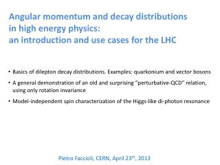
Basics of dilepton decay distributions. Examples: quarkonium and vector bosons A general demonstration of an old and surprising “ perturbative -QCD” relation, using only rotation invariance Model-independent spin characterization of the Higgs-like di -photon resonance.

E N D
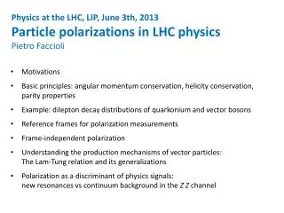
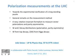
Basics of dilepton decay distributions. Examples: quarkonium and vector bosons A general demonstration of an old and surprising “perturbative-QCD” relation,using only rotation invariance Model-independent spin characterization of the Higgs-like di-photon resonance Angular momentum and decay distributionsin high energy physics: an introduction and use cases for the LHC PietroFaccioli, CERN, April 23th, 2013
Why should we study particle polarizations? • testofperturbative QCD [ZandWdecaydistributions] • constrain universal quantities [sinθWand/orproton PDFsfromZ/W/ * decays] • acceleratediscoveryofnewparticlesorcharacterizethem[Higgs, Z’, anomalousZ+, graviton, ...] • understand the formation of hadrons (non-perturbative QCD)
3/34 Example: formationofψ and • We want to know the relative contributions of the following processes,differing for how/when the observed Q-Qbar bound state acquires its quantum numbers colour-singlet state J = 1 • Colour-singlet processes:quarkonia produceddirectly as observablecolour-neutralQ-Qbar pairs red antired purely perturbative + analogous colour combinations red antired • Colour-octet processes: quarkonia are produced through colouredQ-Qbar pairs ofany possible quantum numbers J = 1 colour-octet state J = 0, 1, 2, … green antiblue Transition to the observable state. Quantum numbers change! J can change! polarization! perturbative non-perturbative
Polarization of vector particles J = 1 → three Jzeigenstates1, +1 ,1, 0 ,1, -1 wrt a certain z Measure polarization = measure (average) angular momentum composition Method: study the angular distribution of the particle decay in its rest frame The decay into a fermion-antifermion pair is an especially clean case to be studied The shape of the observable angular distribution is determined by a few basic principles: 1) “helicity conservation” = 2) rotational covarianceof angular momentum eigenstates f * , Z, g, ... NO YES z' 1, +1 3) parity properties 1 1 1 1, +1 + 1, 1 1, 0 2 2 √2 z ?
1: helicity conservation EW and strong forces preserve the chirality (L/R) of fermions. In the relativistic (massless) limit, chirality = helicity = spin-momentum alignment → the fermion spin never flips in the coupling to gauge bosons: f * , Z, g, ... YES NO YES NO
example: dilepton decay of J/ψ z' 1, M’ℓ+ℓ (–1/2) +1/2 c ( ) ℓ+ ℓ+ ( ) J/ψ rest frame: c * z J/ψ 1, MJ/ψ ( ) (–1/2) ℓ ( ) +1/2 ℓ J/ψangular momentum component alongthepolarizationaxisz: MJ/ψ = -1, 0, +1 (determinedbyproductionmechanism) Thetwoleptonscan onlyhave total angular momentumcomponent M’ℓ+ℓ = +1 or -1along their common direction z’ 0 is forbidden
2: rotation of angular momentum eigenstates z' change of quantization frame: R(θ,φ): z → z’ y → y’ x → x’ Jz’ eigenstates J, M’ θ,φ z + J J, M Σ J, M’ =DMM’(θ,φ)J, M J M = - J Jz eigenstates Wigner D-matrices z' 1, +1 Example: 90° z 1 1 1 1, +1 + 1, 1 1, 0 Classically, we wouldexpect1, 0 2 2 √2
example: M = 0 z' J/ψ (MJ/ψ= 0) →ℓ+ℓ(M’ℓ+ℓ = +1) ℓ+ 1, +1 J/ψ rest frame θ z 1,0 ℓ → the Jz’eigenstate1, +1 “contains” the Jzeigenstate1, 0 with component amplitude D0,+1(θ,φ) 1 → the decay distribution is 1 |D0,+1(θ,φ)|2 = ( 1 cos2θ) |1, +1 |O1, 0|2 1* 1, +1 =D1,+1(θ,φ)1, 1 + D0,+1(θ,φ) 1, 0 + D+1,+1(θ,φ) 1, +1 1 1 1 2 z ℓ+ℓ← J/ψ
ℓ+ ℓ+ 3: parity θ θ z z 1,+1 1,1 1,1 and 1,+1 distributions are mirror reflections of one another ℓ ℓ z z • |D+1,+1(θ,φ)|2 • 1 + cos2θ+ 2cos θ • 1 + cos2θ 2cos θ • |D1,+1(θ,φ)|2 1* 1* Decay distribution of 1,0 stateis always parity-symmetric: Are they equally probable? • 1 + cos2θ+ 2[P(+1)P (1)] cos θ • 1 cos2θ z z z dN dN dN dN z dΩ dΩ dΩ dΩ P (1) > P(+1) P (1) = P(+1) P (1) < P(+1) • |D0,+1(θ,φ)|2 1*
“Transverse” and “longitudinal” z “Transverse” polarization, like for real photons. The word refers to the alignment of the field vector, not to the spin alignment! J/ψ = 1,+1 or 1,1 1 + cos2θ x (parity-conserving case) y z “Longitudinal” polarization J/ψ = 1,0 1 – cos2θ x dN dN y dΩ dΩ
Why “photon-like” polarizations are common We can apply helicity conservation at the production vertex to predict that all vector states produced in fermion-antifermion annihilations (q-q or e+e–) at Born level have transverse polarization q-q rest frame = V rest frame q ( ) (–1/2) +1/2 ( ) ( ) q z V • V = 1,+1 • (1,1) V = *, Z, W q q ( ) The “natural” polarization axis in this case is the relative direction of the colliding fermions (Collins-Soper axis) 1 . 5 Drell-Yan 1 . 0 Drell-Yan is a paradigmatic case But not the only one (2S+3S) 0 . 5 E866, Collins-Soper frame dN 0 . 0 dΩ 1 +λcos2θ - 0 . 5 0 1 2 pT [GeV/c]
The most general distribution z z chosenpolarization axis θ ℓ + production plane φ y x particle rest frame average polar anisotropy average azimuthal anisotropy correlation polar - azimuthal parity violating
Polarization frames zHX zHX zHX zGJ zGJ Helicity axis (HX): quarkonium momentum direction Gottfried-Jacksonaxis (GJ):direction of one or the other beam zCS Collins-Soperaxis (CS): average of the two beam directions h1 h2 Perpendicular helicity axis (PX): perpendicular to CS hadron collision centre of mass frame h2 h2 h2 h1 h1 h1 production plane p zPX particle rest frame particle rest frame particle rest frame
Framedependence For |pL| << pT , the CS and HX frames differ by a rotation of 90º z z′ helicity Collins-Soper 90º x x′ y y′ longitudinal “transverse” (pure state) (mixedstate)
Allreference frames are equal…but some are more equalthanothers What do different detectors measure with arbitrary frame choices? • Gedankenscenario: • dileptons are fully transversely polarized in the CS frame • the decay distribution is measured at the (1S) massby 6 detectors with different dilepton acceptances:
The lucky frame choice (CS in this case) dN 1 +cos2θ dΩ
Less lucky choice (HX in this case) +1/3 λθ = +0.65 λθ = 0.10 1/3 artificial (experiment-dependent!) kinematic behaviour measure in more than one frame!
Frames for Drell-Yan, Z and W polarizations • polarization is always fully transverse... V = *, Z, W _ Due to helicity conservation at the q-q-V(q-q*-V)vertex, Jz = ± 1 along the q-q (q-q*) scattering direction z _ z • ...but with respect to a subprocess-dependent quantization axis _ _ q z = relative dir. of incoming q and qbar ( Collins-Soper frame) q q V important only up to pT = O(partonkT) V q z = dir. of one incoming quark ( Gottfried-Jackson frame) q V q* q* g QCD corrections q V z = dir. of outgoing q (= parton-cms-helicity lab-cms-helicity) q* g q
“Optimal” frames for Drell-Yan, Z and W polarizations Different subprocesses have different “natural” quantization axes q For s-channel processes the natural axis is the direction of the outgoing quark (= direction of dilepton momentum) V q* g q • (neglecting parton-parton-cms • vs proton-proton-cms difference!) • optimal frame (= maximizing polar anisotropy): HX example: Z y = +0.5 HX CS PX GJ1 GJ2 (negative beam) (positive beam) 1/3
“Optimal” frames for Drell-Yan, Z and W polarizations Different subprocesses have different “natural” quantization axes V q q V For t- and u-channel processes the natural axis is the direction of either one or the other incoming parton ( “Gottfried-Jackson” axes) q* q* g • optimal frame: geometrical average of GJ1 and GJ2 axes = CS (pT < M) and PX (pT > M) _ q example: Z y = +0.5 HX CS PX GJ1 = GJ2 MZ 1/3
A complementaryapproach:frame-independent polarization The shape of the distribution is (obviously) frame-invariant (= invariant by rotation) → it can be characterized by frame-independent parameters: z λθ = –1 λφ = 0 λθ = +1 λφ = 0 λθ = –1/3 λφ = –1/3 λθ = +1/5 λφ = +1/5 λθ = +1 λφ = –1 λθ = –1/3 λφ = +1/3 rotations in the production plane
Reducesacceptance dependence Gedankenscenario: vector state produced in this subprocess admixture: 60%processes with natural transverse polarization in the CS frame 40%processes with natural transverse polarization in the HX frame assumed indep. of kinematics, for simplicity CS HX M = 10 GeV/c2 polar azimuthal • Immune to “extrinsic” kinematic dependencies • less acceptance-dependent • facilitates comparisons • useful as closure test rotation- invariant
Physical meaning: Drell-Yan, Z and W polarizations • polarization is always fully transverse... V = *, Z, W _ Due to helicity conservation at the q-q-V(q-q*-V)vertex, Jz = ± 1 along the q-q (q-q*) scattering direction z _ z • ...but with respect to a subprocess-dependent quantization axis q _ _ “natural” z = relative dir. of q and qbar λθ(“CS”)= +1 q q V ~ ~ ~ λ = +1 wrtanyaxis:λ = +1 λ = +1 ~ V q z = dir. of one incoming quark λθ(“GJ”)= +1 q V λ = +1 q* q* any frame g (LO) QCD corrections z = dir. of outgoing q λθ(“HX”)= +1 q V q* ~ N.B.: λ = +1 in both pp-HX and qg-HX frames! g q In all these cases the q-q-V lines are in the production plane (planar processes); The CS, GJ, pp-HX and qg-HX axes only differ by a rotation in the production plane
~ λθvsλ Example: Z/*/W polarization (CS frame) as a function of contribution of LO QCD corrections: Case 2: dominating q-g QCD corrections Case 1: dominating q-qbar QCD corrections pT = 50 GeV/c y = 2 pT = 50 GeV/c pT = 50 GeV/c pT = 50 GeV/c (indep. of y) pT = 200 GeV/c y = 2 pT = 200 GeV/c 1 pT = 200 GeV/c pT = 200 GeV/c (indep. of y) y = 0 y = 0 y = 2 y = 2 0 . 5 y = 0 y = 0 ~ ~ ~ ~ ~ M = 150 GeV/c2 M = 80 GeV/c2 M = 150 GeV/c2 M = 80 GeV/c2 λ = +1 λ = +1 λ = +1 λ = +1 λ = +1 ! mass dependent! 0 fQCD fQCD fQCD fQCD • depends on pT , y and mass • by integrating we lose significance • is far from being maximal • depends on process admixture • need pQCD and PDFs 0 1 0 2 0 3 0 4 0 5 0 6 0 7 0 8 0 λθCS W by CDF&D0 λθ “unpolarized”? No, ~ λ is constant, maximal and independent of process admixture pT [GeV/c]
~ λθvsλ Example: Z/*/W polarization (CS frame) as a function of contribution of LO QCD corrections: Case 2: dominating q-g QCD corrections Case 1: dominating q-qbar QCD corrections pT = 50 GeV/c y = 2 pT = 50 GeV/c pT = 50 GeV/c pT = 50 GeV/c (indep. of y) pT = 200 GeV/c y = 2 pT = 200 GeV/c pT = 200 GeV/c pT = 200 GeV/c (indep. of y) y = 0 y = 0 y = 2 y = 2 y = 0 y = 0 ~ ~ ~ ~ M = 150 GeV/c2 M = 80 GeV/c2 M = 150 GeV/c2 M = 80 GeV/c2 λ = +1 λ = +1 λ = +1 λ = +1 mass dependent! fQCD fQCD fQCD fQCD ~ On the other hand, λ forgets about the direction of the quantization axis. This information is crucial if we want to disentangle the qg contribution, the only one resulting in a rapidity-dependentλθ Measuring λθ(CS) as a function of rapidity gives information on the gluon content of the proton
The Lam-Tung relation A fundamental result of the theory of vector-boson polarizations (Drell-Yan, directly produced Z and W) is that, at leading order in perturbative QCD, independently of the polarization frame Lam-Tung relation, PRD 18, 2447 (1978) This identity was considered as a surprising result of cancellations in the calculations Today we know that it is only a special case of general frame-independent polarization relations, corresponding to a transverse intrinsic polarization: It is, therefore, simply a consequence of 1) rotational invariance 2) properties of the quark-photon/Z/W coupling Experimental tests of the LT relation are not tests of QCD!
Beyond the Lam-Tung relation Even when the Lam-Tung relation is violated, can always be defined and is always frame-independent → Lam-Tung. New interpretation: only vector boson – quark – quarkcouplings (in planar processes) automatically verified in DY at QED & LO QCD levels and in several higher-order QCD contributions → vector-boson – quark – quarkcouplings in non-planar processes (higher-order contributions) → contribution of different/new couplings or processes (e.g.: Z from Higgs, W from top, triple ZZ coupling, higher-twist effects in DY production, etc…)
Spin characterizationoftheHiggs-likedi-photonresonance z' ±1 g θ T restframe T z g ±1 Usual approach to “determine” the J of T: comparison between J=0 hypothesis and ONE alternative hypothesis. Example: graviton with minimal-couplings to SM bosons ( “boson helicity conservation”) SM Higgs boson J=2 J=0 + + OR OR OR OR Mgg = 0 Mgg = 0 Mgg = 0, ±1, ±2 Mgg = 0, ±1, ±2 Decay distribution calculated case-by-case
Spin characterizationoftheHiggs-likedi-photonresonance z' ±1 g θ T restframe T z g ±1 Usual approach to “determine” the J of T: comparison between J=0 hypothesis and ONE alternative hypothesis. Example: graviton with minimal-couplings to SM bosons ( “boson helicity conservation”) SM Higgs boson J=2 J=0 Mgg = ±2 Mgg = ±2
Likelihood Ratio Approach • Method: • measure distribution of the likelihood ratio between hypothesis A and hypothesis B • here A = SM Higgs (JA = 0), B = a new-physics hypothesis (JB) L decay angular distribution L [B] / L [A] • Ingredients (for each set of A and B hypotheses): • the angular momentum quantum numbers JA and JB • the coupling properties of A and B to initial and final particles (gluons and photons) • calculations of the helicity amplitudes for the production and decay processes • Question addressed: • is the observed resonance more likely to be particle A or particle B? • The answer • may be given unhesitatingly, i.e. L [A] >> L [B], even when neither A nor B coincide with the correct hypothesis • is never conclusive until the whole set of possible models for A and B is explored.Do we know this set of models in a totally model-independent way?As a matter of fact, a very restricted set of “B” models is currently considered
MPC approach MPC = Minimal Physical Constraints • Method: • measure the angular distribution dN 1 + λ2 cos2θ + λ4 cos4θ + λ6 cos6θ + … + λNcosNθ dΩ • Ingredients: • angular momentum conservation • initial gluons and final photons are transversely polarized • no hypothesis on J nor on couplings, no explicit calculations of helicity amplitudes [J=1 hypothesis forbidden by Landau-Yang theorem] The general physical parameter domains of the J=2, 3 and 4 cases are mutually exclusive! And do not include the origin (J=0)!
MPC approach MPC = Minimal Physical Constraints • Method: • measure the angular distribution J = 3 J = 4 J = 0 J = 2 dN 1 + λ2 cos2θ + λ4 cos4θ + λ6 cos6θ + … + λNcosNθ dΩ • Ingredients: • angular momentum conservation • Initial gluons and final photons are transversely polarized • no hypothesis on J nor on couplings, no explicit calculations of helicity amplitudes The cosθ distribution discriminates the spin univocally:
MPC approach MPC = Minimal Physical Constraints • Method: • measure the angular distribution dN 1 + λ2 cos2θ + λ4 cos4θ + λ6 cos6θ + … + λNcosNθ dΩ • Ingredients: • angular momentum conservation • Initial gluons and final photons are transversely polarized • no hypothesis on J nor on couplings, no explicit calculations of helicity amplitudes • This method directly addresses the question: • how much is J? • The answer • is model-independent and can be compared to any theory • is always conclusive, if the measurement is sufficiently precise
LR vs MPC The binary strategy of the LR approach aims at discriminating between two hypotheses: From this point of view, this measurementwould correspond to a J=0 characterization 99% C.L. J = 2 minimally-coupling graviton J=2 In the MPC approach this measurementwould represent an unequivocal spin-0 characterization In the MPC approach it would exclude all models lying outside the ellipse, but it would not exclude J=2, nor J=3! 99% C.L. J=3 J = 0 (SM Higgs)
Further reading • P. Faccioli, C. Lourenço, J. Seixas, and H.K. Wöhri,J/psi polarization from fixed-target to collider energies,Phys. Rev. Lett. 102, 151802 (2009) • HERA-B Collaboration, Angular distributions of leptons from J/psi's produced in 920-GeV fixed-target proton-nucleus collisions,Eur. Phys. J. C 60, 517 (2009) • P. Faccioli, C. Lourenço and J. Seixas,Rotation-invariant relations in vector meson decays into fermion pairs,Phys. Rev. Lett. 105, 061601 (2010) • P. Faccioli, C. Lourenço and J. Seixas,New approach to quarkonium polarization studies,Phys. Rev. D 81, 111502(R) (2010) • P. Faccioli, C. Lourenço, J. Seixas and H.K. Wöhri,Towards the experimental clarification of quarkonium polarization,Eur. Phys. J. C 69, 657 (2010) • P. Faccioli, C. Lourenço, J. Seixas and H. K. Wöhri,Rotation-invariant observables in parity-violating decays of vector particles to fermion pairs,Phys. Rev. D 82, 096002 (2010) • P. Faccioli, C. Lourenço, J. Seixas and H. K. Wöhri,Model-independent constraints on the shape parameters of dilepton angular distributions,Phys. Rev. D 83, 056008 (2011) • P. Faccioli, C. Lourenço, J. Seixas and H. K. Wöhri,Determination of chi_c and chi_b polarizations from dilepton angular distributions in radiative decays,Phys. Rev. D 83, 096001 (2011) • P. Faccioli and J. Seixas, Observation of χc and χb nuclear suppression via dilepton polarization measurements,Phys. Rev. D 85, 074005 (2012) • P. Faccioli,Questions and prospects in quarkonium polarization measurements from proton-proton to nucleus-nucleus collisions,invited “brief review”, Mod. Phys. Lett. A Vol. 27 N. 23, 1230022 (2012) • P. Faccioli and J. Seixas, Angular characterization of the Z Z → 4ℓ background continuum to improve sensitivity of new physics searches,Phys. Lett. B 716, 326 (2012) • P. Faccioli, C. Lourenço, J. Seixas and H. K. Wöhri,Minimal physical constraints on the angular distributions of two-body boson decays,submitted to Phys. Rev. D