Key insight.

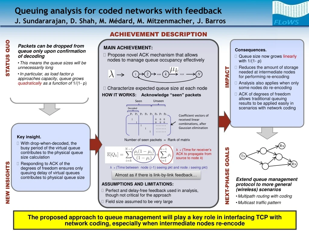
1. ACHIEVEMENT DESCRIPTION STATUS QUO IMPACT NEXT-PHASE GOALS NEW INSIGHTS Queuing analysis for coded networks with feedbackJ. Sundararajan, D. Shah, M. Médard, M. Mitzenmacher, J. Barros • Consequences. • Queue size now grows linearly with 1/(1- ρ) • Reduces the amount of storage needed at intermediate nodes for performing re-encoding • Analysis also applies when only some nodes do re-encoding • ACK of degrees of freedom allows traditional queuing results to be applied easily in scenarios with network coding Packets can be dropped from queue only upon confirmation of decoding • This means the queue sizes will be unnecessarily long • In particular, as load factor ρ approaches capacity, queue grows quadratically as a function of 1/(1- ρ) Unseen • MAIN ACHIEVEMENT: • Propose novel ACK mechanism that allows nodes to manage queue occupancy effectively • Characterize expected queue size at each node Seen λx (Time for receiver’s ACK to propagate from source to node k) Decoded 2 1 k N p1 p2 p3 p4 p5 p6 p7 p8 Coefficient vectors of received linear combinations, after Gaussian elimination HOW IT WORKS: Acknowledge “seen” packets 1 0 0 0 1 0 0 0 1 - - - - - - - 1 - - - - - - - 1 - - - - - - - λx (Time between node (i-1) seeing pkt and node iseeing pkt) • Key insight. • With drop-when-decoded, the busy period of the virtual queue contributes to the physical queue size calculation • Responding to ACK of the degrees of freedom ensures only queuing delay of virtual queues contributes to physical queue size Rx Tx Number of seen packets = Rank of matrix Rx Almost as if there is link-by-link feedback… Extend queue management protocol to more general (wireless) scenarios • Multipath routing with coding • Multicast traffic pattern • ASSUMPTIONS AND LIMITATIONS: • Perfect and delay-free feedback used in analysis, though not critical for the approach • Field size assumed to be very large The proposed approach to queue management will play a key role in interfacing TCP with network coding, especially when intermediate nodes re-encode

2. Problem setup • Tandem network of erasure links • Bernoulli arrival process of rate λ • Perfect delay-free end-to-end feedback (End-to-end nature is motivated by TCP ACKs) • Want to study the expected size of the queues at all the nodes 2 1 k N

3. Questions addressed • With link-by-link feedback (benchmark): • Every link performs simple ARQ – no coding • Every queue behaves like a Geom/Geom/1 queue • Growth of the queue size as load factor ρ→1 is linear in 1/(1-ρ) • With end-to-end feedback: • Need to use intermediate node re-encoding to get to capacity • Degree-of-freedom queue (also called virtual queue) still behaves like a Geom/Geom/1 queue • Can we ensure O(1/(1-ρ)) growth of physical queues in this setting? 2 1 k N

4. Questions addressed • Baseline approach: ACK when decoded • Physical queue size is related to busy period of virtual queues • This gives O(1/(1-ρ)2) growth of queues • Also, this approach causes the delay for decoding at the receiver to enter the round-trip time • This has adverse effects in congestion control – TCP windows will close unnecessarily • Need to ACK every degree of freedom • Then physical queue size will be related to the waiting time for successful transmission • Then we can achieve O(1/(1-ρ)) growth of queues • TCP window will also progress smoothly, since every incoming packet will generate an ACK without waiting for decoding • How to do this in a way that is simple to implement?

5. ‘Seeing’ a packet Seen Unseen Decoded Coefficient vectors of received linear combinations, after Gaussian elimination p1 p2 p3 p4 p5 p6 p7 p8 1 0 0 0 1 0 0 0 1 - - - - - - - 1 - - - - - - - 1 - - - - - - - Witness for p4 Number of seen packets = Rank of matrix = Dim of knowledge space

6. Acknowledge degrees of freedom ACK a packet upon “seeing” it Allows ACK of every innovative linear combination, even if it does not reveal a packet immediately A new kind of ACK Seen Unseen Decoded Coefficient vectors of received linear combinations, after Gaussian elimination p1 p2 p3 p4 p5 p6 p7 p8 1 0 0 0 1 0 0 0 1 - - - - - - - 1 - - - - - - - 1 - - - - - - - Witness for p4

7. The queue update rule • Store every incoming innovative†linear combination • Perform row reduction of the stored coefficient matrix and update the packets correspondingly • Essentially, queue stores witnesses of seen packets • Drop the witness of a packet if you know receiver has seen the packet • Implicit ACK: Although only sender gets receiver’s ACK, other nodes can infer receiver’s state from the sender’s coding window, which is embedded in the header †Innovative means the packet is linearly independent of previously received linear combinations

8. The analysis • Use Little’s law to find the expected queue size using expected time spent in queue • Arrival: Packet arrives into queue of node k when the node first sees the packet • Departure: Packet departs when node k finds out that the receiver has seen the packet • This duration can be broken into two parts: • T1: Time until receiver sees packet • T2: Time till node k learns of receiver’s ACK Lemma: Let SA and SB be the set of packets seen by two nodes A and B respectively. Assume SA\SB is non-empty. Suppose A sends a random linear combination of its witnesses of packets in SA and B receives it successfully. The probability that this transmission causes B to see the oldest packet in SA\SB is (1 − 1/q), where q is the field size.

9. The analysis (contd.) • Lemma implies that the virtual queues behave like a FIFO Geom/Geom/1 queue • Hence, the time between node i seeing a packet and node i+1 seeing the packet is the waiting time in a Geom/Geom/1 queue, with expectation: • Hence, time till receiver sees packet is: • Additional time till receiver’s ACK propagates to node k is • Hence, using Little’s law, the expected queue size is:

10. Conclusions • Proposed a new ACK mechanism that acknowledges every degree of freedom • Analyzed expected queue length for single path with re-encoding at one or more intermediate nodes, and end-to-end feedback • Queue size now grows linearly with 1/(1- ρ) • Need to extend the protocol and analysis to the case of multiple paths and multiple receivers