ASPIRE Class 5 Biostatistics
430 likes | 444 Vues
This class provides an introduction to biostatistics, covering topics such as descriptive and inferential statistics, normal distribution, population and sample, analytic plan, and data collection tools. Learn how to differentiate between different types of data and choose appropriate statistical tests for analysis.

ASPIRE Class 5 Biostatistics
E N D
Presentation Transcript
ASPIRE Class 5Biostatistics • Daniel M. Witt, PharmD, BCPS, FCCP
Learning Objectives ASPIRE Class 5: Biostatistics • Differentiate between descriptive and inferential statistics • Choose an appropriate statistical test based on the type of data being analyzed • Describe the concepts of normal distribution, population, and sample • Formulate the analytic plan for a research study • Evaluate various data collection tools and databases to collect study data
Elements of a Research Protocol Objectives Background Design Population Analytical Plan Procedures
Class 5 Assignment Please come prepared with the above items October 19th, 2:30-5:00 p.m. @ Kaiser Permanente Central Support Services
Why Biostatistics? • Which medical practices actually help? • Determining what therapies are helpful based on simple experience doesn’t work • Biologic variability • Placebo effect
An Example Drug appears to be effective at increasing CO Cardiac output Drug dose
An Example Clearly no relationship between drug dose and CO Cardiac output Drug dose
Biostatistics • A useful tool • Turns clinical and laboratory experience into quantitative statements • Determines whether and by how much a treatment or procedure affected a group of patients • Turns boring data into an interesting story
Learning Point • Experiments rarely include entire population • Selecting unrepresentative samples (bad luck) is unlikely but possible • Biostatistical procedures permit estimation of the chance of such bad luck • Tell a story (who, what, why, where, how)
General Research Goals • Obtain descriptive information about a population based on a sample of that population • Test hypotheses about the population • Minimize bias
Random Variables • Definition: • Outcomes of an experiment or observation whose values cannot be anticipated with certainty • Two types • Discrete • Continuous • “This is important because….” • choosing (and evaluating) statistical methods depends, in part, on the type of data (variables) used
0 1 2 3 Discrete Variables Discrete (counting) Variables • 2 types- • Nominal: classified into groups in no particular order, and with no indication of relative severity (e.g., sex, mortality, disease state, bleeding, stroke, MI) • Ordinal: ranked in a specific order, but with no consistent level of magnitude difference between ranks (e.g., NYHA class, trauma score) Caution: Mean and standard deviation is NOT reported with this type of data
1 Continuous (measuring) Variables • Data are ranked in a specific order with a consistent change in magnitude between units; (e.g., heart rate, LDL cholesterol, blood glucose, INR, blood pressure, time, distance) 2 Continuous Data
Summarizing Data • Bell-shaped frequency distribution • Landmarks • x: mean • SD: standard deviation (SD) Normal distribution: (most common model for population distributions) 30 35 40 45 50 N=200 Mean=40 SD=5.0 x SD SD
N=150 Mean=15 SD=2.5 10 15 20 • Mean (average) • Only used for continuous, normally distributed data • Sensitive to outliers • Most commonly used measure of central tendency
Non-Normal Distributions Mean ± SD N=100 Mean=37.6 SD=4.5 • Although mean and SD can be calculated for any population, • Does not summarize the distribution as well as for normal distributions • A better approach is to use percentiles
Median (50th percentile) • Median • Half of observations fall below and half lie above • Can be used for ordinal or continuous data • Insensitive to outliers
25th percentile 75th percentile • Percentiles • The in a distribution where a value is larger than 25% or 75% of the other values in the sample • Does not assume that the population has a normal distribution
68% 95% - 2SD - 1SD mean + 1SD + 2SD • Standard Deviation (SD) • Appropriately applied only to data that are • normally or near normally distributed • Applicable only to continuous data • Within +/- 1 SD are found 68% of the sample’s values, • Within +/- 2 SD are found 95% of the sample’s values
Hypothesis Testing • The null hypothesis (Ho) • posits no difference between groups being compared (Group A = Group B) • a statistical convention (but a good one) • is used to assist in determining if any observed differences between groups is due to chance alone (bad luck) • in other words, is any observed difference likely due to sampling variation?
Hypothesis Testing • Example: A new anti-obesity medication is compared to an existing one to determine if one agent is better at achieving goal BMI at the recommended starting dose. • Results: Ho:success rate for new drug = success rate for old drug
Hypothesis Testing • Tests for statistical significance determine if the data are consistent with Ho • If Ho is “rejected” = statistically significant difference between groups (unlikely due to chance or ‘bad luck’) • If Ho is “accepted” = no statistically significant difference between groups (results may be due to ‘bad luck’)
Hypothesis Testing • The distribution (range of values) for statistical tests when Ho is true is known • Depending on this statistic’s value, Ho is accepted or rejected • Choosing the appropriate statistical test depends on: • Type of data (nominal, ordinal, continuous) • Study design (parallel, cross-over, etc.) • presence of Confounding variables
Hypothesis Testing 0.05 0.01 0 C2 3.84 6.64 • For our example, • data is nominal data, parallel design with no confounders • appropriate test is C2 • The frequency distribution of C2 when Ho is true is shown above
Hypothesis Testing • Large values are possible when Ho is true, but they occur infrequently (5% of the time when C2 is >3.84 and only 1% of the time when C2 is > 6.64) • These extreme values are used to demarcate the point(s) at which Ho is accepted or rejected
Hypothesis Testing • For our example: • using the data in the formula for calculating C2 yields a value of 1.64 • because 1.64 < 3.84, accept Ho and say that the new drug is not statistically significantly better than the old drug in getting patients to their goal BMI with the recommended starting dose 1.64 0 3.84 C2
Decision Errors The probability of making a Type I error is defined as the significance level a • By setting a at 0.05, this effectively means that 1 out of 20 times a Type I error will occur when Ho is rejected • The calculated probability that a Type I error has occurred is called the “p-value” • When the a level is set a priori, Ho is rejected when p < a
Decision Errors • The probability of making a Type II error (accepting Ho when it should be rejected) is termed b • By convention, b should be < 0.20
Decision Errors Power (1-b) • The ability to detect actual differences between groups • Power is increased by: • Increasing a • Increasing n • Large differences between populations • Power is decreased by: • Poor study design • Incorrect statistical tests
Statistical SignificanceAreas for Vigilance • Size of p-value is not related to the importance of the result • Statistically significant does not necessarily mean clinically significant • Lack of statistical significance does not mean results are unimportant
Choosing a Statistical Test Parametric versus non-parametric • Parametric tests assume an underlying normal distribution • Non-parametric tests: • Non-normally distributed data • Nominal or ordinal data
Choosing a Statistical TestContinuous Data • Student’s t-test • 1 sample: compares mean of study population to the mean of a population whose mean is known • 2 sample (independent samples): compares the means of 2 normal distributions • Paired: compares the means of paired or matched samples
Choosing a Statistical TestContinuous Data • Analysis of variance (ANOVA) • Compares the means of 3 or more groups in a study • Multiple comparison procedures are used to determine which groups actually differ from each other • e.g., Bonferroni, Tukey, Scheffe, others • Analysis of covariance (ANACOVA) • Controls for the effects of confounding variables
These tests may also be used for non-normally distributed continuous data Choosing a Statistical TestOrdinal Data • Wilcoxon rank sum • Mann-Whitney U • Wilcoxon signed rank • Kruskal-Wallis • Friedman
Choosing a Statistical TestNominal Data • X2 • Compares percentages between 2 or more groups • Fisher’s exact test • Infrequent outcomes • McNemar’s • Paired samples • Mantel-Haenszel • Controls for influence of confounders
95% Confidence Intervals • When the ABSOLUTE difference between groups is considered: • A 95% confidence interval that excludes zero is considered statistically significant • The 95% confidence interval also provides information regarding the MAGNITUDE of the difference between groups
Regression • Regression useful in constructing predictive models • Multiple regression involves modeling many possible predictor variables to ascertain which predict a particular target variable • Regression modeling often used to control or adjust for the effects of confounding variables
Example of • predictive modeling • Expected • performance derived • from regression • model Expected performance (99% CI) Observed performance Observed differs from expected by >5% Circ Cardiovasc Qual Outcomes 2011;4:22-29
Survival Analysis • Studies the time between entry into a study and some event (e.g., death) • Takes into account that some subjects leave the study due to reasons other than the ‘event’ (e.g. lost to follow up, study period ends) • May be utilized to arrive at different types of models • Kaplan-Meier • Cox Regression Model • Proportional hazards regression analysis
Kaplan Meier • Uses survival times (or censored survival times) to estimate the proportion of people who would survive a given length of time under the same circumstances • Allows for the production of a survival curve • Uses log-rank test to test for statistically significant differences between groups
1.0 0.8 Treatment 0.6 Cumulative Proportion Surviving 0.4 Control 0.2 0.0 Time Survival Analysis-Kaplan Meier Survival Curve
Cox Regression Modeling • Reported graphically like Kaplan-Meier • Investigates several variables at a time • Allows calculation of relative risk estimate while adjusting for differences between groups