Download
1 / 16
190 likes | 450 Vues
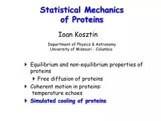
Statistical Mechanics of Proteins. Ioan Kosztin. Department of Physics & Astronomy University of Missouri - Columbia. Equilibrium and non-equilibrium properties of proteins Free diffusion of proteins Coherent motion in proteins: temperature echoes Simulated cooling of proteins.

E N D
Statistical Mechanics of Proteins Ioan Kosztin Department of Physics & Astronomy University of Missouri - Columbia • Equilibrium and non-equilibrium properties of proteins • Free diffusion of proteins • Coherent motion in proteins: temperature echoes • Simulated cooling of proteins
Simulated Cooling of Ubiquitin • Proteins function in a narrow (physiological) temperature range. What happens to them when the temperature of their surrounding changes significantly (temperature gradient) ? • Can the heating/cooling process of a protein be simulated by molecular dynamics ? If yes, then how? • What can we learn from the simulated cooling/heating of a protein ?
Nonequilibrium (Transport) Properties • macromolecular properties of proteins, which are related to their biological functions, often can be probed by studying the response of the system to an external perturbation, such as thermal gradient • “small” perturbations are described by linear response theory (LRT), which relates transport (nonequilibrium) to thermodynamic (equilibrium) properties • on a “mesoscopic” scale a globular protein can be regarded as a continuous medium within LRT, the local temperature distribution T(r,t) in the protein is governed by the heat diffusion (conduction) equation
Atomic vs Mesoscopic • each atom is treated individually • length scale ~ 0.1 Ǻ • time scale ~ 1 fs • one partitions the protein in small volume elements and average over the contained atoms • length scale ≥ 10 Ǻ = 1nm • time scale ≥ 1 ps
0 R r Heat Conduction Equation mass density thermal diffusion coefficient specific heat thermal conductivity • approximate the protein with a homogeneous sphere of radius R~20 Ǻ • calculate T(r,t) assuming initial and boundary conditions:
Thermal diffusion coefficient D=? D is a phenomenological transport coefficient which needs to be calculated either from a microscopic (atomistic) theory, or derived from (computer) experiment “Back of the envelope” estimate: ??? From MD simulation !
Solution of the Heat Equation averaged over the entire protein! protein 1.0 time 0.8 coolant 0.6 0.4 0.2 0 0.2 0.4 0.6 0.8 1
How to simulate cooling ? • In laboratory, the protein is immersed in a coolant and the temperature decreases from the surface to the center • Cooling methods in MD simulations: • Stochastic boundary method • Velocity rescaling (rapid cooling, biased velocity autocorrelation) • Random reassignment of atomic velocities according to Maxwell’s distribution for desired temperature (velocity autocorrelation completely lost)
NAMD User Guide: Temperature Control 6.3 Temperature Control and Equilibration . . . .50 6.3.1 Langevin dynamics parameters . . . . . 6.3.2 Temperature coupling parameters . . . 6.3.3 Temperature rescaling parameters . . . 6.3.4 Temperature reassignment parameters .
Stochastic Boundary Method Heat transfer through mechanical coupling between atoms in the two regions coolant layer of atoms motion of atoms is subject to stochastic Langevin dynamics atoms in the inner region follow Newtonian dynamics δ 2R
2-6-heat_diff: Simulated Cooling of UBQ Start from a pre-equilibrated system of UBQ in a water sphere of radius 26Ǻ mol load psf ubq_ws.psf namdbin ubq_ws_eq.restart.coor Create the a coolant layer of atoms of width 4Ǻ Select all atoms in the system: set selALL [atomselect top all] Find the center of the system: set center [measure center $selALL weight mass] Find X, Y and Z coondinates of the system's center: foreach {xmass ymass zmass} $center { break }
2-6-heat_diff: Simulated Cooling of UBQ Select atoms in the outer layer: set shellSel [atomselect top "not ( sqr(x-$xmass) + sqr(y-$ymass) + sqr(z-$zmass) <= sqr(22) ) "] Set beta parameters of the atoms in this selection to 1.00: $shellSel set beta 1.00 Select the entire system again: set selALL [atomselect top all] Create the pdb file that marks the atoms in the outer layer by 1.00 in the beta column: $selALL writepdb ubq_shell.pdb
NAMD configuration file: ubq_cooling.conf # Spherical boundary conditions # Note: Do not set other bondary conditions and PME if spherical # boundaries are used if {1} { sphericalBC on sphericalBCcenter 30.30817, 28.80499, 15.35399 sphericalBCr1 26.0 sphericalBCk1 10 sphericalBCexp1 2 } # this is to constrain atoms if {1} { constraints On consref ubq_shell.pdb consexp 2 conskfile ubq_shell.pdb conskcol B }
NAMD configuration file: ubq_cooling.conf # this is to cool a water layer if {1} { tCouple on tCoupleTemp 200 tCoupleFile ubq_shell.pdb tCoupleCol B } RUN THE SIMULATION FOR 10 ps (5000 steps; timestep = 2 ps) The (kinetic) temperature T(t) is extracted from the simulation log (output) file; it can be plotted directly with namdplot TEMP ubq_cooling.log Is this procedure of getting T(t) correct ?
300 280 Temperature [K] 260 240 220 0 0.2 0.4 0.6 0.8 1 time [x10ps] Determine D by Fitting the Data