Roots of Equations
Roots of Equations. Bracketing Methods. Root. We are given f ( x ) , a function of x , and we want to find α such that f ( α ) = 0 α is called the root of the equation f ( x ) = 0 , or the zero of the function f ( x ). Example: Interest Rate.


Roots of Equations
E N D
Presentation Transcript
Roots of Equations Bracketing Methods
Root We are given f(x), a function of x, and we want to find α such that f(α) = 0 α is called the root of the equation f(x) = 0, or the zero of the function f(x)
Example: Interest Rate Suppose you want to buy an electronic appliance from a shop and you can either pay an amount of 12,000 or have a monthly payment of 1,065 for 12 months. What is the corresponding interest rate? We know the payment formulae is: A is the monthly payment P is the loan amount x is the interest rate per period of time n is the loan period To find the yearly interest rate, x, you have to find the zero of
Finding Roots Graphically • Not accurate • However, graphical view can provide useful info about a function. • Multiple roots? • Continuous? • etc.
The following root finding methods will be introduced: A. Bracketing Methods A.1. Bisection Method A.2. Regula Falsi (False-position Method) B. Open Methods B.1. Fixed Point Iteration B.2. Newton Raphson's Method B.3. Secant Method
Bracketing Methods Theorem: If a function f(x)is continuous in the interval [a, b]and f(a)f(b) < 0, then the equation f(x) = 0 has at least one real root in the interval (a, b).
Usually • f(a)f(b) > 0implies zero or even number of roots • [figure (a) and (c)] • f(a)f(b) < 0implies odd number of roots • [figure (b) and (d)]
Exceptional Cases • Multiple roots • Roots that overlap at one point. • e.g.: f(x) = (x-1)(x-1)(x-2) has a multiple root at x=1. • Functions that discontinue within the interval
Algorithm for bracketing methods Step 1: Choose two points xl and xu such that f(xl)f(xu) < 0 Step 2: Estimate the root xr (note: xl<xr <xu) Step 3: Determine which subinterval the root lies: if f(xl)f(xr) < 0 // the root lies in the lower subinterval setxuto xrand goto step 2 if f(xl)f(xr) > 0 // the root lies in the upper subinterval setxlto xrand goto step 2 if f(xl)f(xr) = 0 xr is the root
How to select xr in step 2? • Bisection Method Guess without considering the characteristics of f(x) in (xl, xu) • False Position Method (Regula Falsi) Use "average slope" to predict the location of the root
A.1. Bisection Method • Each guess reduce the search interval by half
Bisection Method – Example Find the root of f(x) = 0 with an approximated error below 0.5%. (True root: α=14.7802)
Error Bounds The true root, α, must lie between xl and xu. xl xr xu Let xr(n) denotesxr in the nth iteration After the 1st iteration, the solution, xr(1), should be within an accuracy of xl(1) xu(1) xr(1)
Error Bounds Suppose the root lies in the lower subinterval. xl(2) xr(2) xu(2) xu(1) After the 2nd iteration, the solution, xr(2), should be within an accuracy of
Error Bounds In general, after the nth iteration, the solution, xr(n), should be within an accuracy of If we want to achieve an absolute error of no more than Eα
Implementation Issues • The condition f(xl)f(xr) = 0 (in step 3) is difficult to achieve due to errors. • We should repeat until xr is close enough to the root, but we don't know what the root is! • One possible solution is to estimate the error as and repeat until ea < es (acceptable error)
Bisection Method (as C function) // xl, xu: Lower and upper bound of the interval // es: Acceptable relative percentage error // iter_max: Maximum # of iterations double Bisect(double xl, double xu, double es, int iter_max) { double xr; // Est. root double xr_old; // Est. root in the previous step double ea; // Est. error int iter = 0; // Keep track of # of iterations xr = xl; // Initialize xr in order to // calculating "ea". Can also be "xu". do { iter++; xr_old = xr;
xr = (xl + xu) / 2; // Estimate root if (xr != 0) ea = fabs((xr – xr_old) / xr) * 100; test = f(xl) * f(xr); if (test < 0) xu = xr; else if (test > 0) xl = xr; else ea = 0; } while (ea > es && iter < iter_max); return xr; }
Additional Implementation Issues • Function call is a relatively slow operation. • In the previous example, function f() is called twice in each iteration. Is it necessary? • We only need to update one of the bounds (see step 3 in the algorithm for the bracketing method).
Revised Bisection Method (as C function) double Bisect(double xl, double xu, double es, int iter_max) { double xr; // Est. Root double xr_old; // Est. root in the previous step double ea; // Est. error int iter = 0; // Keep track of # of iterations double fl, fr; // Save values of f(xl) and f(xr) xr = xl; // Initialize xr in order to // calculating "ea". Can also be "xu". fl = f(xl); do { iter++; xr_old = xr; xr = (xl + xu) / 2; // Estimate root fr = f(xr);
if (xr != 0) ea = fabs((xr – xr_old) / xr) * 100; test = fl * fr; if (test < 0) xu = xr; else if (test > 0) { xl = xr; fl = fr; } else ea = 0; } while (ea > es && iter < iter_max); return xr; }
Additional Implementation Issues • Testing if f(xl)f(xr) is positive or negative directly could result in underflow or overflow. • How can we address this problem? • We can test if both the values have the same sign
Comments on Bisection Method • The method is guaranteed to converge. • However, the convergence is slow as we gain only one binary digit in accuracy in each iteration.
A.2. Regula Falsi Method • Also known as the false-position method, or linear interpolation method. • Unlike the bisection method which divides the search interval by half, regula falsi interpolates f(xu) and f(xl) by a straight line and the intersection of this line with the x-axis is used as the new search position. • The slope of the line connecting f(xu) and f(xl) represents the "average slope"(i.e., the value off'(x)) of the points in [xl, xu ].
False-position vs Bisection • False position in general performs better than bisection method. • Exceptional Cases: • (Usually) When the deviation of f'(x) is high and the end points of the interval are selected poorly. • For example,
Bisection Method (Converge quicker) False-position Method
Summary • Bracketing Methods • f(x) has the be continuous in the interval [xl, xu] and f(xl)f(xu) < 0 • Always converge • Usually slower than open methods • Bisection Method • Slow but guarantee the best worst-case convergent rate. • False-position method • In general performs better than bisection method (with some exceptions).