Download
1 / 35
350 likes | 529 Vues
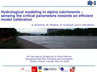
Hydrological modeling in alpine catchments – sensing the critical parameters towards an efficient model calibration. S. Achleitner, M. Rinderer, R. Kirnbauer and H. Kleindienst. 4th International Symposium on Flood Defence: Managing Flood Risk, Reliability and Vulnerability

E N D
Hydrological modeling in alpine catchments – sensing the critical parameters towards an efficient model calibration S. Achleitner, M. Rinderer, R. Kirnbauer and H. Kleindienst 4th International Symposium on Flood Defence: Managing Flood Risk, Reliability and Vulnerability Toronto, Ontario, Canada, May 6-8, 2008
Overview - components of prognosis model • TYROL • Innsbruck • Prognosis model – HoPI • “Hochwasserprognose für den Tiroler Inn
Overview - components of prognosis model • River Inn : 200km from Switzerland to Germany/Bavaria • ~ 60 % of the state area (6700 km2) drain into the River Inn • Innsbruck • Prognosis model – HoPI • “Hochwasserprognose für den Tiroler Inn
Overview - components of prognosis model • River Inn : 200km from Switzerland to Germany/Bavaria • ~ 60 % of the state area (6700 km2) drain into the River Inn • Innsbruck • Largest flood event August 2005 • Innsbruck: 1510 m3/s (HQ100= 1370 m3/s)
Overview - components of prognosis model Tributary catchments Hydrological models River Inn Hydraulic modell Tributary catchments Hydrological models
Overview - components of prognosis model • River INN - Flux/Floris Designer • Hydraulic 1D Model for the River INN • Optimized features for usage in a prognosis system • Implementation of rule based hydropower operation • Driven by external flows from tributary catchments
HoPI • Hydropower power stations – River Inn • Inflows from Reservoir power stations • KW Achensee (28 m3/s) • KW Sellrain Silz (80 m3/s) • KW Imst (85 m3/s) • KW Kaunertal (54 m3/s) • gauge Martina (Switzerland)
Overview – hydrological models • HQsim: 6290 km2 non-glaciated tributary catchments • SES: 460 km2 glaciated tributary catchments • HQsim • 49 modeled catchments • SES • 13 modeled catchments
Overview – Meteorological input to the models • Measurements (online) • HQsim precipitation, temperature >80 stations • SES global radiation, humidity, windspeed > 30 stations • Forecast • INCA - Integrated nowcasting by comprehensive analysis by ZAMG - Central Institute for Meteorology and Geodynamics
Meteoprozessierung • Meteo Forecast: INCA • Mix of numerical weather model (ALADIN) and Nowcasting approach • Spatial resolution (1x1km), Temporal resolution 15min/1h • Nowcasting based on online data in the first 4-6 Stunden • New forecast every hour (Nowcast 1h, Aladin every 6 hours)
HoPI - Data and Information flow INCA Meteo forecast Online measurement WEB-Interface Visualization Model runs Data management - Input, Output, Archive File based System Data processing Spatial and temporal processing of meteo-data, real time control of software components 1x/d 1x/h SES HQsim FLUX
HoPI • HYDROLOGY • Implementation of SES – Snow and Ice melt model • INCA implemented in SES • Verification and correction of meteorological data series • Recalibration of hydrological models • System currently in test phase • Implemented at the Hydrographical Service Tyrol • HYDRAULICS – River INN • Update of Topology new/adapted cross sections • Improve the stability in calculations overcome large gradients in the inflow(low flow conditions/hydropower operation)
Overview - components of prognosis model Brandenberger Ache Area: 280 km² Elevation: 500- 2250 m.a.s.l.
HQsim model background • HQsim – non glaciated catchments • Continuous water balance model • HRU (Hydrologic responce units) conceptderived on basis of • Elevation, Slope, Exposition, • Soil type distribution • Land use
HQsim - parameters • <meteo> • <tempsnowrain><min> • <tempsnowrain><max> • <vegetationtypes> • <sai> • <lai> • <interception><rain> • <soiltypes> • <contributingarea><p1> • <contributingarea><p2> • <contributingarea><imperm> • <evapfactor> • <transfactor> • <topdepth> • <unsat><depth> • <unsat><theta><min> • <unsat><theta><fieldcapacity> • <unsat><theta><max> • <unsat><mvg><ks> • <unsat><mvg><a> • <unsat><mvg><m> • <unsat><drain> • <soil_depth><depth> • <groundwatertypes> • <alpha> • <seepage> • <snowtypes> • <meltfunc><min> • <meltfunc><max> • <tempmemory> • <tempmin> • <groundmelt> • <critdens> • <maxliq> • <surroundingalbedo>
HQsim - parameters • <meteo> • <tempsnowrain><min> • <tempsnowrain><max> • <vegetationtypes> • <sai> • <lai> • <interception><rain> • <vegetationtypes> • <sai> • <lai> • <interception><rain> • <vegetationtypes> • <sai> • <lai> • <interception><rain> • <vegetationtypes> • <sai> • <lai> • <interception><rain> • <vegetationtypes> • <sai> • <lai> • <interception><rain> • <vegetationtypes> • <sai> • <lai> • <interception><rain> • <soiltypes> • <contributingarea><p1> • <contributingarea><p2> • <contributingarea><imperm> • <evapfactor> • <transfactor> • <topdepth> • <unsat><depth> • <unsat><theta><min> • <unsat><theta><fieldcapacity> • <unsat><theta><max> • <unsat><mvg><ks> • <unsat><mvg><a> • <unsat><mvg><m> • <unsat><drain> • <vegetationtypes> • <sai> • <lai> • <interception><rain> • <soiltypes> • <contributingarea><p1> • <contributingarea><p2> • <contributingarea><imperm> • <evapfactor> • <transfactor> • <topdepth> • <unsat><depth> • <unsat><theta><min> • <unsat><theta><fieldcapacity> • <unsat><theta><max> • <unsat><mvg><ks> • <unsat><mvg><a> • <unsat><mvg><m> • <unsat><drain> • <soil_depth><depth> • <soiltypes> • <contributingarea><p1> • <contributingarea><p2> • <contributingarea><imperm> • <evapfactor> • <transfactor> • <topdepth> • <unsat><depth> • <unsat><theta><min> • <unsat><theta><fieldcapacity> • <unsat><theta><max> • <unsat><mvg><ks> • <unsat><mvg><a> • <unsat><mvg><m> • <unsat><drain> • <soil_depth><depth> • <soiltypes> • <contributingarea><p1> • <contributingarea><p2> • <contributingarea><imperm> • <evapfactor> • <transfactor> • <topdepth> • <unsat><depth> • <unsat><theta><min> • <unsat><theta><fieldcapacity> • <unsat><theta><max> • <unsat><mvg><ks> • <unsat><mvg><a> • <unsat><mvg><m> • <unsat><drain> • <soil_depth><depth> • <soiltypes> • <contributingarea><p1> • <contributingarea><p2> • <contributingarea><imperm> • <evapfactor> • <transfactor> • <topdepth> • <unsat><depth> • <unsat><theta><min> • <unsat><theta><fieldcapacity> • <unsat><theta><max> • <unsat><mvg><ks> • <unsat><mvg><a> • <unsat><mvg><m> • <unsat><drain> • <groundwatertypes> • <alpha> • <seepage> • <soil_depth><depth> • <soiltypes> • <contributingarea><p1> • <contributingarea><p2> • <contributingarea><imperm> • <evapfactor> • <transfactor> • <topdepth> • <unsat><depth> • <unsat><theta><min> • <unsat><theta><fieldcapacity> • <unsat><theta><max> • <unsat><mvg><ks> • <unsat><mvg><a> • <unsat><mvg><m> • <unsat><drain> • <groundwatertypes> • <alpha> • <seepage> • <soiltypes> • <contributingarea><p1> • <contributingarea><p2> • <contributingarea><imperm> • <evapfactor> • <transfactor> • <topdepth> • <unsat><depth> • <unsat><theta><min> • <unsat><theta><fieldcapacity> • <unsat><theta><max> • <unsat><mvg><ks> • <unsat><mvg><a> • <unsat><mvg><m> • <unsat><drain> • <groundwatertypes> • <alpha> • <seepage> • <soiltypes> • <contributingarea><p1> • <contributingarea><p2> • <contributingarea><imperm> • <evapfactor> • <transfactor> • <topdepth> • <unsat><depth> • <unsat><theta><min> • <unsat><theta><fieldcapacity> • <unsat><theta><max> • <unsat><mvg><ks> • <unsat><mvg><a> • <unsat><mvg><m> • <unsat><drain> • <groundwatertypes> • <alpha> • <seepage> • <groundwatertypes> • <alpha> • <seepage> • <snowtypes> • <meltfunc><min> • <meltfunc><max> • <tempmemory> • <tempmin> • <groundmelt> • <critdens> • <maxliq> • <surroundingalbedo> • <groundwatertypes> • <alpha> • <seepage> • <groundwatertypes> • <alpha> • <seepage>
HQsim - parameters • Why reducing the parameters? • Too many parameter describing the rainfall-runoff relation • Confusing when calibrating • Auto calibration: less parameters to be considered in a first approach
HQsim model background • HQsim – model specifics • Precipitation types - Snowline modelinglower and upper temperature thresholds (tsrmin/tsrmax) • Snow melt – modified day degree factor approach min and max value of snow melting function (snmfmin,snmfmax) [mm/°C/d] • Snow cover described by “cold content”melting initiated whenS Energy loss < S Energy input Physical limits of “cold content” accumulationsntmem max. days used for Energy balancesntmin min. threshold temp. to be stored
HQsim model background • HQsim – model specifics • Contributing area for surface runoff described as arctan function f (saturation) • (s) saturation • (i) fraction of seald surface • (cap1, cap2) describe the shape of the arctan function
HQsim model background • HQsim – model specifics • Water movement in soil(sd) …soil depth (mvgks) …saturated hydraulic conductivity • Unsaturated hydraulic conductivity (k) Mualem van-Genuchten • (mvkm, mvga) Mualem van-Genuchten parameters
Calibration of hydrological models • AIM: Best reproduction of large flow events
Calibration of hydrological models • AIM: Best reproduction of large flow events • Considering single relevant (large) events • Separation with threshold flow Qmin=~HQ1
Parameter variation • Comparability of parameter variations • % variation based on physical feasible range • [Cmin, Cmax] …physical range of parameter • Pv [%] … percentage of variation applied • C0 … (current) best fit of parameter • CV=f(pv)…Variation of parameter
Indicators for sensitivity • - 30,20,10 % • 0 % • + 10,20,30 %
Indicators for sensitivity • Indicators for Calibration quality = • = indicators for sensitivity • BQ,MAX [-] …Bias of the peak flow • E [-] …Nash Sutcliffe Efficiency (event period) • DQ,MAX [h] …Delay of peak flow • BRL [-] …Bias of the rising limb • ERL [-] …Nash Sutcliffe Efficiency (rising limb) • Indicator for time series • mean of event indicators + standard deviation • Uses the baseline simulation as reference
Results • 1994 - 2001 • BQ,MAX [-] • …Bias of the peak flow
Results • 1994 - 2001 DQ,MAX [h] …Delay of peak flow
Results • 1994 - 2001 E [-]…Nash Suttcliffe Efficiency (event period)
Results • 1994 - 2001 BRL [-] …Bias of the rising limb
Conclusions • Sensitive parameters • (cap1, cap2)describe flow contributing area • (mvgks, mvgm) flow in unsaturated soil zone (Mualem vanGenuchten) • (sd)soild depth of the unsaturated soil zone • Most important (sensitive) parameters were identified • Indicators account on large flow events • Temp/Snow type parameters are relevant only in specific events
thank you for your attention Contact:Stefan Achleitner achleitner@alps-gmbh.com
HQsim model background • HQsim – non glaciated catchments • Derivation of flow paths/river representations • Modeled with linear flow routing • Combination of • River paths • HRU • Flowtimes from HRU 2 flowpaths