Understanding BJT Differential Amplifiers: Analysis & Applications
Learn about BJT differential amplifiers, including large-signal and small-signal analysis, frequency response, noise reduction, common-mode rejection, and more. Explore practical examples and characteristics of differential pairs.

Understanding BJT Differential Amplifiers: Analysis & Applications
E N D
Presentation Transcript
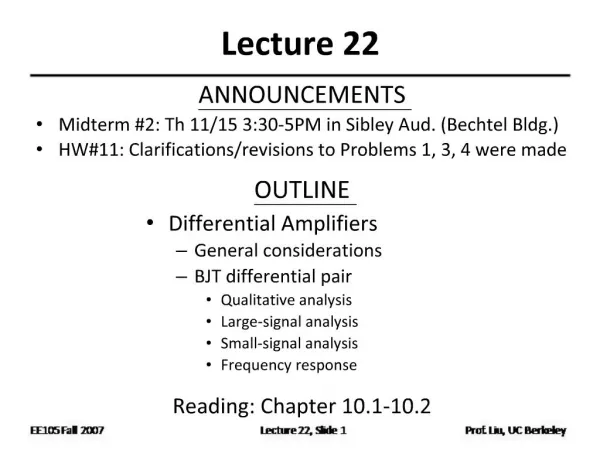
1. Lecture 22 OUTLINE
Differential Amplifiers
General considerations
BJT differential pair
Qualitative analysis
Large-signal analysis
Small-signal analysis
Frequency response
Reading: Chapter 10.1-10.2
2. �Humming� Noise in Audio Amplifier Consider the amplifier below which amplifies an audio signal from a microphone.
If the power supply (VCC) is time-varying, it will result in an additional (undesirable) voltage signal at the output, perceived as a �humming� noise by the user.
3. Supply Ripple Rejection Since node X and Y each see the voltage ripple, their voltage difference will be free of ripple.
4. Ripple-Free Differential Output If the input signal is to be a voltage difference between two nodes, an amplifier that senses a differential signal is needed.
5. Common Inputs to Differential Amp. The voltage signals applied to the input nodes of a differential amplifier cannot be in phase; otherwise, the differential output signal will be zero.
6. Differential Inputs to Differential Amp. When the input voltage signals are 180� out of phase, the resultant output node voltages are 180� out of phase, so that their difference is enhanced.
7. Differential Signals Differential signals share the same average DC value and are equal in magnitude but opposite in phase.
A pair of differential signals can be generated, among other ways, by a transformer.
8. Single-Ended vs. Differential Signals
9. BJT Differential Pair With the addition of a �tail current,� an elegant and robust differential pair is achieved.
10. Common-Mode Response Due to the fixed tail current, the input common-mode value can vary without changing the output common-mode value.
11. Differential Response
12. Differential Response (cont�d)
13. Differential Pair Characteristics A differential input signal results in variations in the output currents and voltages, whereas a common-mode input signal does not result in any output current/voltage variations.
14. Virtual Ground For small input voltages (+DV and -DV), the gm values are ~equal, so the increase in IC1 and decrease in IC2 are ~equal in magnitude. Thus, the voltage at node P is constant and can be considered as AC ground.
15. Extension of Virtual Ground It can be shown that if R1 = R2, and the voltage at node A goes up by the same amount that the voltage at node B goes down, then the voltage at node X does not change.
16. Small-Signal Differential Gain Since the output signal changes by -2gm?VRC when the input signal changes by 2?V, the small-signal voltage gain is �gmRC.
Note that the voltage gain is the same as for a CE stage, but that the power dissipation is doubled.
17. Large-Signal Analysis
18. Input/Output Characteristics
19. Linear/Nonlinear Regions of Operation
20. Small-Signal Analysis
21. Half Circuits Since node P is AC ground, we can treat the differential pair as two CE �half circuits.�
22. Half Circuit Example 1
23. Half Circuit Example 2
24. Half Circuit Example 3
25. Half Circuit Example 4
26. Differential Pair Frequency Response Since the differential pair can be analyzed using its half circuit, its transfer function, I/O impedances, locations of poles/zeros are the same as that of its half circuit.