Regression analysis can be used to develop an
260 likes | 709 Vues
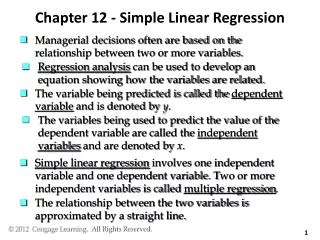
Chapter 12 - Simple Linear Regression. Managerial decisions often are based on the relationship between two or more variables. Regression analysis can be used to develop an equation showing how the variables are related. The variable being predicted is called the dependent

Regression analysis can be used to develop an
E N D
Presentation Transcript
Chapter 12 - Simple Linear Regression • Managerial decisions often are based on the relationship between two or more variables. • Regression analysis can be used to develop an equation showing how the variables are related. • The variable being predicted is called the dependent variable and is denoted by y. • The variables being used to predict the value of the dependent variable are called the independent variables and are denoted by x. • Simple linear regression involves one independent • variable and one dependent variable. Two or more • independent variables is called multiple regression. • The relationship between the two variables is approximated by a straight line.
Simple Linear Regression Model • The equation that describes how y is related to x and • an error term is called the regression model. • The simple linear regression model is: y = b0 + b1x +e where: • b0 and b1 are called parameters of the model, • e is a random variable called the error term.
Simple Linear Regression Equation • The simple linear regression equation is: E(y) = 0 + 1x • Graph of the regression equation is a straight line. • b0 is the y intercept of the regression line. • b1 is the slope of the regression line. • E(y) is the expected value of y for a given x value.
E(y) x Simple Linear Regression Equation • Positive Linear Relationship Regression line Intercept b0 Slope b1 is positive
E(y) x Simple Linear Regression Equation • Negative Linear Relationship Intercept b0 Regression line Slope b1 is negative • You can show No Relationship
is the estimated value of y for a given x value. Estimated Simple Linear Regression Equation • The estimated simple linear regression equation • The graph is called the estimated regression line. • b0 is the y intercept of the line. • b1 is the slope of the line.
Sample Data: x y x1 y1 . . . . xnyn Estimated Regression Equation Sample Statistics b0, b1 Estimation Process Regression Model y = b0 + b1x +e Regression Equation E(y) = b0 + b1x Unknown Parameters b0, b1 b0 and b1 provide estimates of b0 and b1
^ yi = estimated value of the dependent variable for the ith observation Least Squares Method where: yi = observed value of the dependent variable for the ith observation • Least Squares Criterion
Simple Linear Regression Model y Observed Value of y for xi εi Slope = β1 Predicted Value of y for xi Random Error for this xi value Intercept = β0 x Xi
_ x = mean value for independent variable y = mean value for dependent variable _ Least Squares Method where: xi = value of independent variable for ith observation yi = value of dependent variable for ith observation • y-Intercept for the Estimated Regression Equation • Slope for the Estimated Regression Equation
Simple Linear Regression • Example: Reed Auto Sales Reed Auto periodically has a special week-long sale. As part of the advertising campaign Reed runs one or more television commercials during the weekend preceding the sale. Data from a sample of 5 previous sales are shown here. Number of TV Ads (x) Number of Cars Sold (y) 1 3 2 1 3 -1x-6 1x4 0x-2 -1x-3 1x7 14 24 18 17 27 Sx = 10 Sy = 100
Estimated Regression Equation • Slope for the Estimated Regression Equation • y-Intercept for the Estimated Regression Equation • Estimated Regression Equation
Reed Auto Sales Estimated Regression Line Using Excel’s Chart Tools for Scatter Diagram & Estimated Regression Equation
Measures of Variation • Total variation is made up of two parts: Total Sum of Squares Regression Sum of Squares Error Sum of Squares where: = Mean value of the dependent variable yi = Observed value of the dependent variable = Predicted value of y for the given xi value
Measures of Variation • SST = total sum of squares (Total Variation) • Measures the variation of the yi values around their mean y • SSR = regression sum of squares (Explained Variation) • Variation attributable to the relationship between x and y • SSE = error sum of squares (Unexplained Variation) • Variation in y attributable to factors other than x
Measures of Variation y yi y y _ _ y y x xi
Coefficient of Determination r2 or R2 SST = SSR + SSE where: SST = total sum of squares SSR = sum of squares due to regression SSE = sum of squares due to error r2 = SSR/SST = 100/114 = .8772 The regression relationship is very strong; 87.72% of the variability in the number of cars sold can be explained by the linear relationship between the number of TV ads and the number of cars sold. • Relationship Among SST, SSR, SSE
where: b1 = the slope of the estimated regression equation Sample Correlation Coefficient – We learned in Chapter 3
The sign of b1 in the equation is “+”. Sample Correlation Coefficient rxy = +.9366 Note: This only holds for simple regression
Examples of Approximate r2 (or R2) Values Y r2 = 1 Perfect linear relationship between X and Y: 100% of the variation in Y is explained by variation in X X r2 = 1 Y X r2 = 1
Examples of Approximate r2 (or R2) Values Y 0 < r2 < 1 Weaker linear relationships between X and Y: Some but not all of the variation in Y is explained by variation in X X Y X
Examples of Approximate r2 (or R2) Values r2 = 0 Y No linear relationship between X and Y: The value of Y does not depend on X. (None of the variation in Y is explained by variation in X) X r2 = 0