Download
1 / 65
650 likes | 995 Vues
By Cheng Few Lee Joseph Finnerty John Lee Alice C Lee Donald Wort. Chapter 15 Commodity Futures, Financial Futures, and Stock-Index Futures. Outline. 15.1 COMMODITY FUTURES 15.2 FUTURES QUOTATIONS 15.3 FINANCIAL FUTURES 15.3.1 Currency Futures 15.3.1.1Evolution

E N D
By Cheng Few Lee Joseph Finnerty John Lee Alice C Lee Donald Wort Chapter 15Commodity Futures, Financial Futures, and Stock-Index Futures
Outline • 15.1 COMMODITY FUTURES • 15.2 FUTURES QUOTATIONS • 15.3 FINANCIAL FUTURES • 15.3.1 Currency Futures • 15.3.1.1Evolution • 15.3.1.2 Advantages • 15.3.1.3 Pricing Currency Futures • 15.3.2 The Traditional Theory of International Parity • 15.3.2.1 Interest-Rate Parity • 15.3.2.2 Purchasing-Power Parity • 15.3.2.3 Fisherian Relation • 15.3.2.4 Forward Parity
15.3.3 Interest-Rate Futures • 15.3.4 US Treasury Debt Futures • 15.3.4.1 Characteristics of T-Bill Futures • 15.3.4.2 Pricing T-Bill Futures Contracts • 15.3.4.3 Characteristics of T-Note and T-Bond Futures • 15.3.5 The Eurodollar Futures Market • 15.3.5.1 Evolution • 15.3.5.2 Eurodollar Futures • 15.4 STOCK-INDEX FUTURES • 15.4.1 Pricing Stock-Index Futures Contracts • 15.4.2 Stock-Index Futures: Does the Tail Wag the Dog? • 15.5 SUMMARY
15.1 Commodity Futures • Commodity futures contracts were forward agreements for future trade. • The agricultural industry was first because the perishable goods have price risks. • A person can also “lock in” on contracted future price by arranging the expiration date of the contract to be the same as the day it hits the market.
Sample Problem 15.1 • Farmer Smith decided to hedge his price risk by going into the futures market and effectively selling his crop ahead of time. • Assuming there’s no basis risk, the outcomes of this transaction for falling and risking prices over the interim period are shown below. Table 15-1Hedging the Price Risk by Futures Market
Speculatorsbuy the futures contracts from the farmer on the chance that prices would actually rise and now fall as expected. • Speculators contributes to the functioning of futures markets in two invaluable ways: • Risk transference • Liquidity
15.2 Futures Quotations • To find certain future contract, for example corn future, click the item “Core, Oats, Rice” under agriculture here Figure 15.1 Futures Prices Data
Then obtain the corn future price in the figure above. • Table 15.2 shows useful definitions for future contracts. • Commodity trade is corn • Exchange refers to the place where the futures contracts are traded • Contract size refers to the amount of spot commodity that the contract represent • The price is the manner in which the prices are quoted Figure 15.2 Corn Future Prices Table 15.2 Future Terms
15.3 Financial Futures • Financial futures are standardized futures contracts whose market prices are established through open outcry and hand signals in regulated commodity exchange. 15.3.1 Currency Futures • Currency futures contracts promises future delivery of a standard amount of a foreign currency at a specified time, place, and price. • It can be used to hedge foreign-exchange risk for investors and firms involved in the import and export business.
15.3.1.1 Evolution • The concept of financial futures on currencies emerged as an anticipatory reaction to the end of the Bretton Woods Agreement, which called for elimination of fixed parities between major currencies. • On May 16, 1972, the International Monetary Market (IMM) and Mercantile Exchange (CME) opened and offered the first organized trading of standardized futures contracts on foreign currencies. • The change in U.S. monetary policy in October1979, which went from essentially “pegging” interest rates to letting them float in accordance with market forces, resulted in a significant increase in the volatility of market interest rates. • As interest rates change in one country, so does the value of its currency relative to those of other counties.
15.3.1.2 Advantages • The establishment of currency futures has provided a means by which Interbank dealers can hedge their positions in spot or forward markets. • The funds of participants are protected by daily settlement of the change in position values; they are also safeguarded by the exchange’s clearing house, whose members together guarantee all trades. • Futures markets allow dealers to trade anonymously and provide price insurance and arbitrage opportunities in the spot and forward markets. • The IMM (International Monetary Market)is today one of three divisions of the CME, the largest futures exchange in the United States. • Presently, the foreign currencies for which futures contracts are traded include U.K. pound (ticker code GBP); Canadian dollars (CAD); Euro (EUR); Swiss franc (CHF); Japanese yen (JPY); Russian Ruble (RUB); and Australian dollar (AUD).
When dealing with foreign exchange, it is important to realize that the price of a currency is in terms of a second currency. • Both the numerator and denominator of the price ratio are in terms of money. Figure 15.3 Currency Futures Data
For example, in Figure 15-4 the euro is worth $1.2663 (0.7897 dollar per euro) and the yen is worth $0.0117 (85.22 Yen per dollar). • All foreign-exchange rates are related as reciprocals. • For other currencies (usually the currencies of the major trading nations), not only are the spot rates quoted but also the forward rates. Figure 15.4 Currency Rates
The futures market is different from the forward market. In the futures market, the maturity date of a given contract is fixed by the rules of the exchange. • In the forward market, 30-, 60-, and 90-day contracts (or any other number of days) are available. • In the forward market, the contract size is determined between the buyer and seller. • In the futures market, only contracts of standardized amounts are traded.
15.3.1.3 Pricing Currency Futures • The arbitrage argument used to establish the price of a currency futures contract relative to the spot price is called interest-rate parity. • In the case of the U.S. dollar/British pound: • Where • = equilibrium price at time t for a currency futures contract maturing at time T; • = spot price at time t for the foreign currency (to which the futures contract applies); • = US interest rate on risk-free securities maturing at time T; and • = British interest rate on risk-free securities maturing at time T. (15.1)
Sample Problem 15.2 • As an example, suppose the US dollar is currently quoted in the spot currency market for the British pound at $1.80/£. • Interest rates in the United States and Britain for three months are 3% and 4%, respectively. • What is the price of a three-month deposit futures contract for pounds? Solution: Substituting all information into Equation (15.1): Empirical tests have shown that the pricing relationship described by interest-rate parity holds very closely in the currency markets.
Spot prices of foreign currency were described as following a random walk, where money incorporates anticipations of its future value into its current value, an example is how the future stock prices and dividend estimates are reflected in today’s stock price. • Using this rational-expectations hypothesis and momentarily assuming no inventory costs: or, today’s price reflects the expected price for the foreign currency at time T. • Equation (15.2) can be reversed: • Hence, the best estimate for the spot price at some future point in time T is the current spot price of the currency. • Since the currency-futures price at time t for a contract maturing at time T reflects the expected spot price for the foreign currency at time T: , or = • Without carrying costs, the current futures price = current spot price for any foreign currency. (15.2) (15.3) (15.4)
Sample Problem 15.3 • Transactions and closing position value: January 1, 1989 Buy $1.3 million worth of pounds. Invest proceeds at 10-% British rate. Sell £1 million worth of futures at $1.33. January 1, 1990 Proceeds from earned interest $150,000 Deliver £1 million against short futures Position at $1.33/£1.00 $1,330,000 Gross revenue $1,460,000 Less initial investment $1,300,000 Net profit $160,000 Annual return 12.3%
From all these transactions the investor earns an annualized return of 12.3% on the original investment of $1.3 million. • This return is composed of the interest earned on the riskless British-government security and the 0.03 difference in spot and one-year futures prices for the pound (i.e., the investor sold the pound at $1.33 but only paid $1.30). • If the investor can borrow U.S. dollars at a rate less than 12.3%, then a riskless arbitrage opportunity is available. • All pressures discussed in this problem will continue until the arbitrage opportunity has dissipated, which is when: = • interest rates on securities with the same maturity as the futures contract (in this case, one year). (15.6)
Rearrange Equation (15.6) to solve for the futures price for a one-year contract on British pounds, we have = • This is the interest-rate parity relationship from Equation (15.1). • Thus, the equilibrium one-year futures price for British pounds that would eliminate the arbitrage opportunity in the example can be computed as = = (15.7)
15.3.2 The Traditional Theory of International Party • The writings of Keynes, Cassel, and Irving Fisher implicitly require four conditions for international currency parity. • Financial markets are perfect. There are no controls, transaction costs, taxes, and so on. • Goods markets are perfect. Shipment of goods anywhere in the world is costless. • There is a single consumption good common to everyone. • The future is known with certainty.
15.3.2.1 Interest-Rate Parity • For any two countries, the difference in their domestic interest rates must be equal to the forward exchange-rate differential: = • where = the interest rate for countries i and j, respectively, in time t; = the forward exchange rate of currency iin units of currency j quoted at time t for delivery at t + 1; and = the spot exchange rate of currency i in units of currency j at time t. • Based on only the first assumption.
15.3.2.2 Purchasing-Power Parity • Based on first and third assumptions, the purchasing-power parity theorem says that a given currency has the same purchasing power in every country: = • where = the spot rate between countries i and j at time t; and and = price level in countries iand j at time t, respectively.
15.3.2.3 Fisherian Relation • Based on first, third, and fourth assumption, the Fisherian relation says that the nominal interest rate in every country will be equal to the real rate of interest plus the expected future inflation rate: (1 + ) = (1 + )(1 + ), • where = the real rate of interest in country j at time t; = the nominal rate of interest at time t; and = the inflation rate at time t. • The implication of this relationship is that if the real rate of interest is equal everywhere, then the inflation differential between countries is fully reflected in their nominal interest rates.
15.3.2.4 Forward Parity • The forward exchange rate ( ) must be equal to the spot exchange rate at some future point in time ( ): = • This relationship (forward parity) must be true given the first three relationships derived above; otherwise, arbitrage opportunities would exist. • Sample Problem 15.4 will demonstrate.
Sample Problem 15.4 • Note that I + = / . Then, assuming that 1 + = 1 + , it follows that • which is equal to 1 plus the rate of currency appreciation (or depreciation). • The linkages among interest rates, price levels, expected inflation, and exchange rates are all relevant in pricing a currency contract.
15.3.3 Interest-Rate Futures • Financial futures-related, interest-rate-sensitive instruments such as US Treasury debt futures are the focus of this section. • Sample daily price quotations for interest-rate futures are shown in Figure 15.5. Figure 15.5 Interest Rate Futures Data Source:The Wall Street Journal, August 24, 2010
15.3.4 U.S. Treasury Debt Futures • The US Treasury issues debt securities, which are backed by the government and are considered to be free of default risk, to finance government operations and the federal deficit. • The debt can be classified into 3 types based on its time to maturity: • US Treasury bills (T-bills), with a time to maturity of one year • US Treasury notes (T-notes), with a time to maturity of between one year and 10 years • US Treasury bonds (T-bonds), with a time to maturity of more than 10 years • One of the attractive features of US Treasury securities is that they can easily be resold, because a strong secondary market exists for them. • T-bill futures are traded at the IMM, while T-notes futures and T-bond futures are offered by the CBT.
15.3.4.1 Characteristics of T-Bill Futures • T-bills (as well as T-notes and T-bonds) are traditionally quoted in terms of their yield to maturity. • Since interest rates (or yields) and prices of debt securities move inversely, the common perception that a long position makes money as the quoted values increase does not apply to such instruments. • The IMM quote system for its interest-rate securities is essentially an index based on the difference between the actual T-bill price and 100.00. • When the IMM T-bill futures contract reaches the maturity date, the seller of the contract may have to make delivery of the underlying T-bill.
Figure 15.6 Delivery of an IMM T-Bill Futures Contract • Figure 15.6 illustrates the delivery process. • The major function of the clearinghouse is to see that the transfer and payment (4B and 4S in Figure 15-6) take place in a timely fashion. • Should either party default in any way, the clearinghouse will complete the transaction and then seek to recover from the defaulting party.
15.3.4.2 Pricing T-Bill Futures Contracts • Consider the situation of an investor faced with the following choice. (1) Invest in a 182-day T-bill, or (2) Invest in a 91-day T-bill and buy a futures contract maturing 91 days hence. • In a perfectly efficient market, the investor should be indifferent between these equivalent investments, since both offer the same return. • Now let = yield on a 91-day T-bill, m = 1 = yield on a 182-day T-bill, m = 2 = yield on a futures contract maturing m days from now = implied forward rate on a T-bill with a life equal to n– m • If the market is to be in equilibrium, then: = = (1 + ). (15.8)
Investing in a 91-day T-bill and then buying a futures contract maturing in 91 more days is equal to initially investing in a 182-day T-bill. • Arbitrage conditions will arise if < > • To compute , the implied forward rate of a T-bill with a life of n − m, the following example is utilized. • Assume that the 182-day T-bill rate is 11% and the three-month T-bill rate is 10%. The implied three-month forward rate is then: - 1 = - 1 (15.9)
If an arbitrager observed that the futures rate was above 12% (or had a price less than 88.00), he or she could profit from the following strategy. • Borrow money at 11% (assuming lending and borrowing rates are equal) by selling short a six-month T-bill. • Buy a three-month T-bill. • Simultaneously, buy one T-bill futures contract with a time to maturity of three months. • Combining the spot and futures T-bill positions results in a synthetic six-month T-bill with a yield exceeding that realized on the actual six-month T-bill. • For instance, if the futures contract has a rate of 15%, the six-month annualized return on the synthetic position is = 11.48%
Arbitrage profit is equal to the realized yield on the synthetic position minus the cost of establishing that position. • Based on past few examples, the theoretical price for a T-bill future can be derived from Equation (15.8). • First, by taking its inverse: • or, equivalently: • where is the price of an n-day T-bill paying $1 at maturity. And, therefore: = price of a T-bill futures contract, quoted as the difference between $100 and the annualized discount from par assuming 360 days in a year = spot price of an n-day T-bill = spot price of an m-day T-bill (n > m) (15.11) (15.12) (15.13)
Equation (15.13) can be altered to account for transaction costs such as commissions and a greater than zero bid-ask dealer spread (or bid-offer). • In doing so the boundary conditions for the price of a T-bill futures contract are obtained: CC= round-trip commission costs per $100 of face value = the price at which a dealer will sell an n-day T-bill = the price at which a dealer will buy an m-dayT-bill
Sample Problem 15.5 • Using Equation (15.13), compute the theoretical futures price for the IMM December 1989 contract as of June 7, 1988. • Assume that the deliverable bill (in period) against the futures contract is the T-bill maturing March 21, 1989, with a bid price of 10.67 and ask price of 10.59. • Also assume $0.004 per $100 of face value as the round-trip commission cost.
Solution: • Determine the T-bill rate corresponding to the m period — the interval between June 7, 1989, and the third Thursday of December 1989, the delivery date of the contract (i.e., m = 188 days). • Find the price of this T-bill maturing in (approximately) 188 days (December 27) from the US T-bill data listed earlier. Its bid price is 10.47 and its ask price is 10.41. • Now calculate without commission costs using Equation (15.13) and an average of the bid and ask prices for the m period and n period and n-period T-bills. = = 0.97053 • To get the quarterly yield (price) for the futures 100 – 97.053 = 2.947
Annualized yield: 2.947 x = 11.658 • Theoretical future price = 100 – 11.658 = 88.342 • When you compare this price with the market price of 88.32 for the December 1989 T-bill future contract, you see that it’s upwardly biased. • This disparity could be due to neglect of transaction costs such as commissions; so you would calculate it on an annualized basis but take it out from the computed price. 0.004 x = 0.016 And = 88.342 – 0.016 = 88.326
15.4.3 Characteristics of T-Note and T-Bond Futures • T-bond futures as on the CBT require the delivery of a US T-bond with a face value of $100,000 and maturing at least 15 years from maturity. • Prices are quoted as a percentage of par in the same way as GNMA futures prices are quoted. • The depth of trading in this contract is revealed by the existence of outstanding T-bond contracts with maturities nearly three years into the future. • T-note futures is growing in popularity and also offered by CBT. • One of the underlying stimuli for its success is the growing proportion of total Treasury debt, which is represented by T-note securities. • The T-note futures contract specifies the delivery of a US Treasury note with a face value of $100,000 and a maturity of no less than 6.5 years and no more than 10 years form the date of delivery.
Figure 15.7 Contract Specification of T-Bonds and T-Notes Futures Source: CME Group, U.S. Treasury Bond Futures and 2-Year U.S. Treasury Note Futures
15.3.5 The Eurodollar Futures Market • A Eurodollar is any dollar on deposit outside the United States. • An important aspect of these deposits is that, because of their location outside of the United States they do not fall under US jurisdiction. • Therefore, Eurodollars are not governed by the same regulations that apply to domestic deposits, set by the Federal Reserve. 15.3.5.1 Evolution • The Eurodollar market evolved in the 1950s in response to Federal Reserve restrictions on the maximum allowable interest rate to be paid on a deposit. • Because Foreign merchants didn’t have this restriction, they were earning more money, so US banks eventually allowed their London branches to enter that market and take in dollar deposits.
As the Eurodollar markets developed and matured, formal lines of credit and sovereign risk limitations were formalized by participants. • A bank lending funds in the Eurodollar market is exposed to essentially three risks: • The interest-rate risk involved with a Eurodollar loan is the same as before • Credit riskis a larger concern in the Eurodollar market because of the difficulties that can arise when trying to analyze a foreign borrower’s financial position • Sovereign risk is unique to the arena of international lending; it refers to the unfavorable consequences that can have impact on a bank’s investment if a foreign government is overthrown, becomes economically unstable, or passes detrimental regulations affecting the movement of funds • Most banks will have sovereign-risk limitations restricting the total amount placed on deposit with (or loaned to) institutions in any one country.
The relationship between three-month rates offered on Eurodollar deposits (as measured by the London Interbank Offered Rate (LIBOR) rate), US CDs, and US T-bills can be visualized for a two-year period in Figure 15.8. • Few things on the relationships can be noted from the chart. • Eurodollar rates are higher than CD rates, which are higher than T-bill rates — a ranking consistent with the level of risk inherent in these securities. • The variation in the spread between Eurodollar rates and CD rates are affected by a variety of unpredictable market forces and decisions of US and foreign government. • Unlike the behavior of the spread between Eurodollar and CD rates, the Eurodollar rates and Treasury rates have a less predictable tendency to rise together as rates rise. Figure 15.8 Three-Month Rates on U.S. CDs, U.S. T-Bills, and Eurodollar deposits, Jan 2007 – Jan 2010 (monthly data) Source: Board of Governors of the Federal Reserve System https://www.federalreserve.gov/default.htm
15.3.5.2 Eurodollar Futures • Eurodollar futures are traded on the Chicago Mercantile Exchange (CME) (Figure 15-9) and the London International Financial Exchange (LIFFE). • The primary use of Eurodollar futures as a hedging vehicle is similar to that of other hedging vehicles; they are capable of protecting against detrimental changes in interest rates. Figure 15.9 Eurodollar Futures Quotes Source: CME Group, March 10, 2011, http://www.cmegroup.com/
The Eurodollar futures contract has as its underlying instrument a three-month Eurodollar time deposit in the amount of $1 million as shown in Figure 15.10. Figure 15.10 Eurodollar Futures Contract Source: CME Group http://www.cmegroup.com/
Sample Problem 15.7 • Suppose that the London branch of a US bank anticipates a decline in rates from September 16 to December 16. • Furthermore, on June 12, the bank makes a three-month loan in the Eurodollar market and finances the loan with the funds from a six-month Eurodollar CD. • The process in which the bank loans and borrow money makes it prone to reinvestment-rate risk. • To alleviate the problem, the bank chooses to fix the reinvestment rate for the latter three-month investment horizon through a long position in Eurodollar Futures. • On June 12, the Eurodollar contract for September delivery was priced at an index of 86.53 (100% − 13.47%), the six-month Eurodollar CD rate was 13%, and the initial three-month loan was made at the LIBOR rate of 14%. • Table 15.3 summarizes the transactions results.
As Table 15.3 indicates, the use of the futures position to hedge the interest-rate risk allows the bank to reduce its reinvestment rate loss by 71%. Table 15.3 Hedging Interest Rate Risk by Future Market
15.4 Stock-Index Futures • Stock-index futures offer the investor a medium for expressing an opinion on the general course of the market, and these contracts can be used by portfolio managers in a variety of ways to alter the risk-return distribution of their stock portfolios. • The calculation of the market value for a stock-index futures contract on any given day is simply a matter of multiplying the current index price for the contract by the appropriate dollar amount. • Each of the US stock-index futures is listed in order of market popularity. • Each contract bought and sold on a particular day is included in the calculation of daily trading volume. • Open interest represent the number of open contract positions on a given day with only one side counted — that is, when the buyer and seller make their transaction, only one position is counted as being open, not two.
Figure 15.11 shows prices, volume, and open interest for S&P 500 indexes future. Figure 15.11 S&P 500 Future Quotes Source: The Wall Street Journal, August 23, 2010
Figure 15.12 S&P 500 Future Contract Source: GME Group, http://www.cmegroup.com/