Lecture 8: Hidden Markov Models (HMMs)

1. Lecture 8:Hidden Markov Models (HMMs) Prepared by Michael Gutkin Shlomi Haba Originally presented at Yaakov Stein’s DSPCSP Seminar, spring 2002 Modified by Benny Chor, using also some slides of Nir Friedman (Hebrew Univ.), for the Computational Genomics Course, Tel-Aviv Univ., Dec. 2002

2. Hidden Markov Models – Computational Genomics Outline • Discrete Markov Models • Hidden Markov Models • Three major questions: • Q1. Computing the probability of a given observation. A1. Forward – Backward (Baum Welch) DP algorithm. • Q2. Computing the most probable sequence, given an observation. A2. Viterbi DP Algorithm • Q3. Given an observation, learnbest model. A3. Expectation Maximization (EM): A Heuristic.

3. Hidden Markov Models – Computational Genomics Markov Models • A discrete (finite) system: • N distinct states. • Begins (at time t=1) in some initial state. • At each time step (t=1,2,…) the system moves from current to next state (possibly the same as the current state) according to transition probabilities associated with current state. • This kind of system is called aDiscrete Markov Model

4. Hidden Markov Models – Computational Genomics Discrete Markov Model • Example: Discrete Markov Model with 5 states • Each of the aij represents the probability of moving from state i to state j • The aij are given in a matrix A = {aij} • The probability to start in a given state i is pi , The vector p represents these startprobabilities.

5. Hidden Markov Models – Computational Genomics Types of Models • Ergodic model Strongly connected - directed path w/ positive probabilities from each state i to state j (but not necessarily complete directed graph)

6. Hidden Markov Models – Computational Genomics Types of Models (cont.) • Left-to-Right (LR) model • Index of state non-decreasing with time

7. Hidden Markov Models – Computational Genomics Discrete Markov Model - Example • States – Rainy:1, Cloudy:2, Sunny:3 • Matrix A – • Problem – given that the weather on day 1 (t=1) is sunny(3), what is the probability for the observation O:

8. Hidden Markov Models – Computational Genomics Discrete Markov Model – Example (cont.) • The answer is -

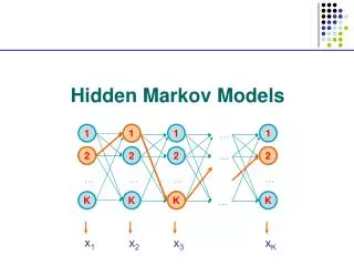
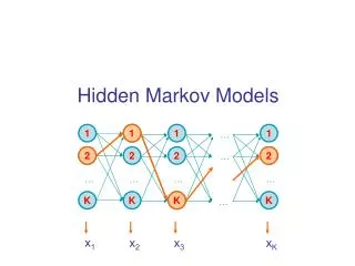
9. Hidden Markov Models – Computational Genomics a11 a44 a33 a22 a12 a34 a23 b14 b11 b13 b12 4 1 3 2 Hidden Markov Models (probabilistic finite state automata) Often we face scenarios where states cannot be directly observed. We need an extension: Hidden Markov Models aij are state transition probabilities. bik are observation (output) probabilities. Observed phenomenon b11 + b12 + b13 + b14 = 1, b21 + b22 + b23 + b24 = 1, etc.

10. Hidden Markov Models – Computational Genomics Example: Dishonest Casino Actually, what ishidden in this model?

11. Hidden Markov Models – Computational Genomics Biological Example: CpG islands • In human genome, CpG dinucleotides are relatively rare • CpG pairs undergo a process called methylation that modifies the C nucleotide • A methylated C can (with relatively high probability) mutate to a T • Promoter regions are CpG rich • These regions are not methylated, and thus mutate less often • These are called CpG islands

12. Hidden Markov Models – Computational Genomics CpG Islands • We construct two Markov chains: One for CpG rich, one for CpG poor regions. • Using observations from 60K nucleotide, we get two models, + and - .

13. Hidden Markov Models – Computational Genomics HMMs – Question I • Given an observation sequence O= (O1 O2 O3 … OT), and a model M = {A, B, p}, how do we efficiently compute P(O|M), the probability that the given model M produces the observation O in a run of length T ? • This probability can be viewed as a measure of the quality of the model M. Viewed this way, it enables discrimination/selection among alternative models.

14. Hidden Markov Models – Computational Genomics HMM – Question II (Harder) • Given an observation sequence, O =(O1 O2 O3 … OT), and a model, M = {A, B, p }, how do we efficiently compute the most probable sequence(s) of states, Q? • That is, the sequence of states Q=(Q1 Q2 Q3 … QT),which maximizes P(O|Q,M), the probability that the given model M produces the given observation O when it goes through the specific sequence of states Q. • Recall that given a model M,a sequence of observations O, and a sequence of states Q, we can efficiently compute P(O|Q,M) (should watch out for numeric underflows)

15. Hidden Markov Models – Computational Genomics HMM – Question III (Hardest) • Given an observation sequence O =(O1 O2 O3 … OT),and a class of models, each of the form M = {A, B, p }, which specific model “best” explains the observations? • A solution to question I enables the efficient computation of P(O|M) (the probability that a specific modelM produces the observation O). • Question III can be viewed as a learning problem: We want to use the sequence of observations in order to “train” an HMM and learn the optimal underlying model parameters (transition and output probabilities).

16. Hidden Markov Models – Computational Genomics HMM Recognition (question I) • For a given model M = { A, B, p} and a given state sequence Q1 Q2 Q3 … QT ,, the probability of an observation sequence O1 O2 O3 … OT is P(O|Q,M) =bQ1O1 bQ2O2 bQ3O3 …bQTOT • For a given hidden Markov model M = { A, B, p} the probability of the state sequence Q1 Q2 Q3 … QT is (the initial probability ofQ1 is taken to bepQ1) P(Q|M) =pQ1aQ1Q2aQ2Q3aQ3Q4…aQT-1QT • So, for a given hidden Markov model, M the probability of an observation sequence O1 O2 O3 … OT is obtained by summing over all possible state sequences

17. Hidden Markov Models – Computational Genomics HMM – Recognition (cont.) P(O| M) = S P(O|Q) P(Q|M) = SQpQ1bQ1O1 aQ1Q2bQ2O2 aQ2Q3bQ2O2 … • Requires summing over exponentially many paths • But can be made more efficient

18. Hidden Markov Models – Computational Genomics ~ ~ HMM – Recognition (cont.) T • Why isn’t it efficient? – O(2TQ ) • For a given state sequence of length T we have about 2T calculations • P(Q|M) = pQ1aQ1Q2aQ2Q3aQ3Q4…aQT-1QT • P(O|Q) = bQ1O1bQ2O2bQ3O3…bQTOT • There are Q possible state sequence • So, if Q=5, and T=100, then the algorithm requires 2 100 5 1.6 10 computations • We can use the forward-backward (F-B) algorithm T 100 72 x x x

19. Hidden Markov Models – Computational Genomics The F-B Algorithm • Some definitions 1. Legal final state – a state at which a path through the model may end. 2. a - a “forward-going” 3. b – a “backward-going” 4. a(j|i) = aij ; b(O|i) = biO 5. O = the observation O1O2…Otin times 1,2,…,t (O1 on t=1, O2 on t=2, etc.) t 1

20. Hidden Markov Models – Computational Genomics The F-B Algorithm (cont.) • a can be recursively calculated • Stopping condition • Moving from state i to state j • But we can enter state j from all others states

21. Hidden Markov Models – Computational Genomics The F-B Algorithm (cont.) • Now we can work sequentially • And on time t=T we get what we wanted -

22. Hidden Markov Models – Computational Genomics The F-B Algorithm (cont.) • The full algorithm – Run Demo

23. Hidden Markov Models – Computational Genomics The F-B Algorithm (cont.) • The likelihood is measured using any sequence of states of length T • This is known as the “Any Path” Method • We can choose an HMM by the probability generated using the best possible sequence of states • We’ll refer to this method as the “Best Path” Method

24. Hidden Markov Models – Computational Genomics Most Probable States Sequence (ques. II) Idea: • If we know the value of Qi , then the most probable sequence on i+1,…,n does not depend on observations before time i • Let Vl(i) be the probability of the best sequence Q1,…,Qisuch that Qi = l

25. Hidden Markov Models – Computational Genomics Viterbi Algorithm • A DP problem • Grid • X – frame index, t (time) • Q – State index, i • Constraints • Every path must advance in time by one, and only one, time step for each path segment • Final grid points on any path must be of the form (T, if ), where if is a legal final state in a model

26. Hidden Markov Models – Computational Genomics Viterbi Algorithm (cont.) • Cost • Node (t,i) – the probability to emit the observation y(t) on state i =biy • Transition from (t-1,i) to (t,j) – the probability to change state from i to j = aij • The total cost associated with the path is given by the product of the costs (type B) • Initial Transition cost: a0i = pi • Goal • The best path will be the one of maximum cost

27. Hidden Markov Models – Computational Genomics Viterbi Algorithm (cont.) • We can use the trick of taking negative logarithms • Multiplications of probabilities are expansive and numerically problematic • Sums of numerically stable numbers are simpler • The problem is turned into a minimal-cost path search

28. Hidden Markov Models – Computational Genomics Run Demo Viterbi Algorithm (cont.)

29. Hidden Markov Models – Computational Genomics HMM – EM Training • Using the Baum-Welch algorithm • Is an EM algorithm • Estimate – approximate the result • Maximize – and if needed, re-estimate • The estimation algorithm is based on DP algorithms (F-B & Viterbi)

30. Hidden Markov Models – Computational Genomics HMM – EM Training (cont.) • Initializing • Begin with an arbitrary model M • Estimate • Evaluate the likelihood P(O|M) • Along the way, keep track of some tallies • Recalculate the matrixes A and B • e.g, aij= • Maximize • If P(O|M) – P(O|M) ≥ e, re-estimate with M=M • Use several initial models to find a favorable local maximum of P(O|M) number of transitions from i to j number of transitions exiting state i

31. Hidden Markov Models – Computational Genomics HMM – Training (cont.) • Why a local maximum?

32. Hidden Markov Models – Computational Genomics Auxiliary Physiology Model

33. Hidden Markov Models – Computational Genomics Auxiliary cont. Articulation

34. Hidden Markov Models – Computational Genomics Patterson - Barney Diagram Mapping by the formants Auxiliary cont. Spectrogram