Forecasting

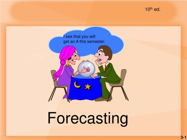
1. I see that you willget an A this semester. 10th ed. Forecasting

2. FORECAST: • A statement about the future value of a variable of interest such as demand. • Forecasting is used to make informed decisions. • Long-range • Short-range

3. Features of Forecasts • Assumes causal systempast ==> future • Forecasts rarely perfect because of randomness • Forecasts more accurate forgroups vs. individuals • Forecast accuracy decreases as time horizon increases

5. Uses of Forecasts • Forecasts affect decisions and activities throughout an organization • Accounting, finance • Human resources • Marketing • MIS • Operations • Product / service design

6. Examples of Forecasting Uses

7. Elements of a Good Forecast Timely Accurate Reliable Easy to use Written Meaningful

8. Steps in the Forecasting Process “The forecast” Step 6 Monitor the forecast Step 5 Make the forecast Step 4 Obtain, clean and analyze data Step 3 Select a forecasting technique Step 2 Establish a time horizon Step 1 Determine purpose of forecast

9. Types of Forecasts • Judgmental - uses subjective inputs (e.g., sales force estimates). • Time series - uses historical data assuming the future will be like the past. Time could be in weeks, months, years, etc., and is based on t=1,2,3,… • Associative models - uses explanatory variables to predict the future. It suggests a causal relationship, such as personal consumption being based on per capita income of households.

10. Judgmental Forecasts • Executive opinions • Sales force opinions • Consumer surveys • Outside opinion • Delphi method • Opinions of managers and staff • Achieves a consensus forecast

11. Time Series Forecasts • Trend - long-term movement in data • Seasonality - short-term regular variations in data • Cycle – wavelike variations of more than one year’s duration • Irregular variations - caused by unusual circumstances that are not random • Random variations - caused by chance

12. Forecast Variations Irregularvariation Trend Cycles 90 89 88 Seasonal variations

15. Some Common Time Series Techniques or Time Series Forecasting Models • Naïve forecasts • Moving average • Weighted moving average • Exponential smoothing

16. Naive Forecasts The forecast for any period equals the previous period’s actual value.

17. Naïve Forecasts • Simple to use • Virtually no cost • Quick and easy to prepare • Data analysis is nonexistent • Easily understandable • Cannot provide high accuracy • Can be a standard for accuracy

18. Formula for Naïve Forecasts • Ft = At-1 This is the forecasting that is the most responsive to changes in the past actual demand.

19. Moving Average Formula • Moving average – A technique that averages a number of recent actual values, updated as new values become available. • Weighted moving average – More recent values in a series are given more weight in computing the forecast. At-n+ … At-2 + At-1 Ft = MAn= n Ft = WMAn= wnAt-n+ … wn-1At-2 + w1At-1

20. Simple Moving Average At-1 + At-2+ … At-n Ft = MAn= n Actual Demand MA5 MA3

21. Exponential Smoothing • Weighted averaging method based on previous forecast plus a percentage of the forecast error • A-F is the error term,  is the % feedback Ft = Ft-1 + (At-1 - Ft-1)

22. Exponential Smoothing Formula • Premise--The most recent observations might have the highest predictive value. • Therefore, we should give more weight to the more recent time periods when forecasting. • The symbol “α” is the Greek letter “alpha.” Alpha is called the smoothing constant. Note that alpha varies from zero to one. Ft = Ft-1 + (At-1 - Ft-1)

23. Exponential Smoothing

24. Picking a Smoothing Constant Actual .4  .1

26. Homework Problem Referring to page 118 in the text, do problems 2a and 2b, but skip problem 2b(1) which asks for a linear trend equation. Complete and partial solutions of homework problems are found on the slides at the end of this session. For this problem and for all homework problems, do not go to the solutions until you have made a strong effort tosolve the problems.

27. Linear Trend Equation Ft 0 1 2 3 4 5 t • Ft = Forecast for period t • t = The time period being forecasted • a = Value of Ft at t = 0 • b = Slope of the line Ft = Yt = a + bt

28. Calculating a and b n (ty) - t y    b = 2 2 n t - ( t)   y - b t   a = n Yt = a + bt where b and a follow from the following formulae:

29. Linear Trend Equation Example Calculations of b and a are from the sums given in the table on the left. Ft = Yt = a + bt n = 10 Ft = Yt = a + bt = 67.78 + 5.79t

30. Plot of Previous Slide Y t

31. Homework Problem Referring to page 118 in the text, do 2b(1), which asks for a linear trend equation. Also,do problem 2c. However, change problem 2c to read as follows: “Which method seems MOST appropriate?Why?”

32. Associative Forecasting • Associative models - uses explanatory variables to predict the future. It suggests a causal relationship, such as personal consumption being based on per capita income of households

33. Example of an Associative Forecast: Using x to Predict y Computedrelationship A straight line is fitted to a set of sample points.

34. Example of an Associative Forecast Equation for Automobiles (with several variables, and nonlinear)

35. Forecast Accuracy • Error - difference between actual value and predicted value • Mean Absolute Deviation (MAD) • Average absolute error • Mean Squared Error (MSE) • Average of squared error

36. Some Measures of Forecasting Accuracy 2 ( Actual  forecast)  MSE = n - 1   Actual forecast MAD = n Note that the errors are taken for each of the past n periods where the actual demand is known.

37. Some Characteristics of MAD and MSE • MAD • Easy to compute • Weights errors linearly • MSE • Squares error • More weight to large errors

38. Sources of Forecast errors • Model may be inadequate • Irregular variations • Incorrect use of forecasting technique

39. In-class assignment The next two slides ask some basic questions about forecasting, and give some examples of measuring forecasting error. These slides make up an in-class assignment. You can try to answer the questions on the slides. However, if you have difficulty with all or some of the questions, we will do them in class. At least become familiar with the questions before the next class. If you find the next two slides difficult to read, simply magnify the size of the slides. If you can, please try to print a hardcopy of the next two slides and bring them to class. If you can set the resolution of your printer, it is suggested that you set it to a high resolution for the best printed copy.

42. Choosing a Forecasting Technique • No single technique works in every situation • Two most important factors • Cost • Accuracy • Other factors include the availability of: • Historical data • Computers • Time needed to gather and analyze the data • Forecast horizon

43. Good Operations Strategy • Understand that forecasts are the basis for many decisions • Work to improve short-term forecasts • Understand that accurate short-term forecasts have benefits for the following: • Profits • Lower inventory levels • Reduce inventory shortages • Improve customer service levels • Enhance forecasting credibility

44. Supply Chain Forecasts • Sharing forecasts with suppliers can • Improve forecast quality in the supply chain • Lower costs • Lead to shorter lead times

45. Common Nonlinear Trends Parabolic Exponential Growth

46. Exponential Smoothing

47. Linear Trend Equation

48. Simple Linear Regression

49. Sales 20 0 F M A M J J A S Month Homework Problem Solutions 2a

50. 2b(1) To solve this problem, we need to plug the appropriate values into the equation Ft = Yt = a + bt Hence, n = 7, t = 28, t2 = 140 Therefore, Yt = 16.86 + .50t For the September forecast, t = 8, and Yt = 16.86 + .50(8) = 20.86