Visibility Algorithms
Visibility Algorithms. Jian Huang, CS594, Fall 2001 This set of slides reference slides used at Ohio State for instruction by Prof. Machiraju and Prof. Han-Wei Shen. Visibility Determination. AKA, hidden surface elimination. Hidden Lines. Hidden Lines Removed. Hidden Surfaces Removed.

Visibility Algorithms
E N D
Presentation Transcript
Visibility Algorithms Jian Huang, CS594, Fall 2001 This set of slides reference slides used at Ohio State for instruction by Prof. Machiraju and Prof. Han-Wei Shen.
Visibility Determination • AKA, hidden surface elimination
Topics • Backface Culling • Hidden Object Removal: Painters Algorithm • Z-buffer • Spanning Scanline • Warnock • Atherton-Weiler • List Priority, NNA • BSP Tree • Taxonomy
y clipped line x 1 y 1 near far clipped line x z 0 1 z image plane near far Where Are We ? • Canonical view volume (3D image space) • Clipping done • division by w • z > 0
Back-face Culling • Problems ? • Conservative algorithms • Real job of visibility never solved
Back-face Culling • If a surface’s normal is pointing to the same direction as our eye direction, then this is a back face • The test is quite simple: if N * V > 0 then we reject the surface
Painters Algorithm • Sort objects in depth order • Draw all from Back-to-Front (far-to-near) • Is it so simple?
3D Cycles • How do we deal with cycles? • Deal with intersections • How do we sort objects that overlap in Z?
Form of the Input Object types: what kind of objects does it handle? • convex vs. non-convex • polygons vs. everything else - smooth curves, non-continuous surfaces, volumetric data
Form of the output Precision: image/object space? • Object Space • Geometry in, geometry out • Independent of image resolution • Followed by scan conversion • Image Space • Geometry in, image out • Visibility only at pixels
Object Space Algorithms • Volume testing – Weiler-Atherton, etc. • input: convex polygons + infinite eye pt • output: visible portions of wireframe edges
Image-space algorithms • Traditional Scan Conversion and Z-buffering • Hierarchical Scan Conversion and Z-buffering • input: any plane-sweepable/plane-boundable objects • preprocessing: none • output: a discrete image of the exact visible set
Conservative Visibility Algorithms • Viewport clipping • Back-face culling • Warnock's screen-space subdivision
Z-buffer • Z-buffer is a 2D array that stores a depth value for each pixel. • InitScreen: for i := 0 to N dofor j := 1 to N doScreen[i][j] := BACKGROUND_COLOR; Zbuffer[i][j] := ; • DrawZpixel (x, y, z, color)if (z <= Zbuffer[x][y]) thenScreen[x][y] := color; Zbuffer[x][y] := z;
Z-buffer: Scanline I. foreach polygondoforeach pixel (x,y) in the polygon’s projectiondoz := -(D+A*x+B*y)/C; DrawZpixel(x, y, z, polygon’s color); II. foreach scan-liney doforeach “in range” polygon projectiondo for each pair (x1, x2) of X-intersections dofor x := x1 to x2doz := -(D+A*x+B*y)/C; DrawZpixel(x, y, z, polygon’s color); If we know zx,y at (x,y) than: zx+1,y = zx,y - A/C
Incremental Scanline On a scan line Y = j, a constant Thus depth of pixel at (x1=x+Dx,j) , since Dx = 1,
Incremental Scanline (contd.) • All that was about increment for pixels on each scanline. • How about across scanlines for a given pixel ? • Assumption: next scanline is within polygon , since Dy = 1,
P3 P4 P2 ys za zp zb P1 Non-Planar Polygons Bilinear Interpolation of Depth Values
Non Trivial Example ? Rectangle: P1(10,5,10), P2(10,25,10), P3(25,25,10), P4(25,5,10) Triangle: P5(15,15,15), P6(25,25,5), P7(30,10,5) Frame Buffer: Background 0, Rectangle 1, Triangle 2 Z-buffer: 32x32x4 bit planes
Z-Buffer Advantages • Simple and easy to implement • Amenable to scan-line algorithms • Can easily resolve visibility cycles
Z-Buffer Disadvantages • Does not do transparency easily • Aliasing occurs! Since not all depth questions can be resolved • Anti-aliasing solutions non-trivial • Shadows are not easy • Higher order illumination is hard in general
Spanning Scan-Line Can we do better than scan-line Z-buffer ? • Scan-line z-buffer does not exploit • Scan-line coherency across multiple scan-lines • Or span-coherence ! • Depth coherency • How do you deal with this – scan-conversion algorithm and a little more data structure
Spanning Scan Line Algorithm • Use no z-buffer • Each scan line is subdivided into several "spans" • Determine which polygon the current span belongs to • Shade the span using the current polygon’s color • Exploit "span coherence" : • For each span, only one visibility test needs to be done
Spanning Scan Line Algorithm • A scan line is subdivided into a sequence of spans • Each span can be "inside" or "outside" polygon areas • "outside“: no pixels need to be drawn (background color) • "inside“: can be inside one or multiple polygons • If a span is inside one polygon, the pixels in the span will be drawn with the color of that polygon • If a span is inside more than one polygon, then we need to compare the z values of those polygons at the scan line edge intersection point to determine the color of the pixel
Determine a span is inside or outside (single polygon) • When a scan line intersects an edge of a polygon • for a 1st time, the span becomes "inside" of the polygon from that intersection point on • for a 2nd time, the span becomes "outside“ of the polygon from that point on • Use a "in/out" flag for each polygon to keep track of the current state • Initially, the in/out flag is set to be "outside" (value = 0 for example). Invert the tag for “inside”.
When there are multiple polygon • Each polygon will have its own in/out flag • There can be more than one polygon having the in/out flags to be "in" at a given instance • We want to keep track of how many polygons the scan line is currently in • If there are more than one polygon "in", we need to perform z value comparison to determine the color of the scan line span
Z value comparison • When the scan line is intersecting an edge and leaving a new polygon, we then use the color of the reminding polygon if there is now only 1 polygon "in". If there are still more than one polygon with "in" flag, we need to perform z comparison only when the scan line is leaving a non-obscured polygon
Many Polygons ! • Use a PT entry for each polygon • When polygon is considered Flag is true ! • Multiple polygons can have flag set true ! • Use IPL as active In-Polygon List !
Example Think of ScanPlanes to understand !
Spanning Scan-Line: Example Y AET IPL I x0, ba , bc, xN BG, BG+S, BG II x0, ba , bc, 32, 13, xN BG, BG+S, BG, BG+T, BG III x0, ba , 32, ca, 13, xN BG, BG+S, BG+S+T, BG+T, BG IV x0, ba , ac, 12, 13, xN BG, BG+S, BG, BG+T, BG
Some Facts ! • Scan Line I: Polygon S is in and flag of S=true • ScanLine II: Both S and T are in and flags are disjointly true • Scan Line III: Both S and T are in simultaneously • Scan Line IV: Same as Scan Line II
Spanning Scan-Line build ET, PT -- all polys+BG polyAET := IPL := Nil; for y := yminto ymaxdo e1 := first_item ( AET );IPL := BG;while (e1.x <> MaxX) doe2 := next_item (AET); poly := closest poly in IPL at [(e1.x+e2.x)/2, y] draw_line(e1.x, e2.x, poly-color);update IPL (flags); e1 := e2;end-while;IPL := NIL; update AET;end-for;
Depth Coherence ! Depth relationships may not change between polygons from one scan-line to scan-line These can be kept track using the AET and PT How about penetrating polygons
Penetrating Polygons Y AET IPL I x0, ba , 23, ad, 13, xN BG, BG+S, S+T, BG+T,BG I’ x0, ba , 23, ec, ad, 13, xN BG, BG+S, BG+S+T, BG+S+T, BG+T, BG False edges and new polygons!
Area Subdivision 1 (Warnock’s Algorithm) Divide and conquer: the relationship of a display area and a polygon after projection is one of the four basic cases:
Warnock : One Polygon if it surrounds then draw_rectangle(poly-color); else begin if it intersects then poly := intersect(poly, rectangle); draw_rectangle(BACKGROUND); draw_poly(poly); end else; What about contained and disjoint ?
Warnock’s Algorithm • Starting from the entire display area, we check the following four cases. If none holds, we subdivide the area, otherwise, we stop and perform the action associated with the case • All polygons are disjoint wrt the area -> draw the background color • Only 1 intersecting or contained polygon -> draw background, and then draw the contained portion of the polygon • There is a single surrounding polygon -> draw the entire area in the polygon’s color • There are more than one intersecting, contained, or surrounding polygons, but there is a front surrounding polygon -> draw the entire area in the polygon’s color • The recursion stops when you are at the pixel level
At Single Pixel Level • When the recursion stop and none of the four cases hold, we need to perform depth sort and draw the polygon with the closest Z value • The algorithm is done at the object space level, except scan conversion and clipping are done at the image space level
Warnock : Zero/One Polygons warnock01(rectangle, poly) new-poly := clip(rectangle, poly); if new-poly = NULL then draw_rectangle(BACKGROUND); elsedraw_rectangle(BACKGROUND); draw_poly(new-poly); return;
Warnock(rectangle, poly-list) new-list := clip(rectangle, poly-list); if length(new-list) = 0 then draw_rectangle(BACKGROUND); return; if length(new-list) = 1 then draw_rectangle(BACKGROUND); draw_poly(poly); return; if rectangle size = pixel size then poly := closest polygon at rectangle center draw_rectangle(poly color); return; warnock(top-left quadrant, new-list); warnock(top-right quadrant, new-list); warnock(bottom-left quadrant, new-list); warnock(bottom-right quadrant, new-list);